Learning Dynamics of the Complex Valued Neural Network in the Neighborhood of Singular Points

(1)

http://dx.doi.org/10.4236/jcc.2014.21005

Learning Dynamics of the Complex-Valued Neural

Network in the Neighborhood of Singular Points

Tohru Nitta

National Institute of Advanced Industrial Science and Technology (AIST), Tsukuba, Japan. Email: [email protected]

Received December 4th_{, 2013; revised December 28}th_{, 2013; accepted January 4}th_{, 2014}

Copyright © 2014 Tohru Nitta. This is an open access article distributed under the Creative Commons Attribution License, which permits unrestricted use, distribution, and reproduction in any medium, provided the original work is properly cited. In accordance of the Creative Commons Attribution License all Copyrights © 2014 are reserved for SCIRP and the owner of the intellectual property Tohru Nitta. All Copyright © 2014 are guarded by law and by SCIRP as a guardian.

ABSTRACT

In this paper, the singularity and its effect on learning dynamics in the complex-valued neural network are elu-cidated. It has learned that the linear combination structure in the updating rule of the complex-valued neural network increases the speed of moving away from the singular points, and the complex-valued neural network cannot be easily influenced by the singular points, whereas the learning of the usual real-valued neural network can be attracted in the neighborhood of singular points, which causes a standstill in learning. Simulation results on the learning dynamics of the three-layered real-valued and complex-valued neural networks in the neighbor-hood of singularities support the analytical results.

KEYWORDS

Complex-Valued Neural Network; Complex Number; Learning; Singular Point

1. Introduction

Complex-valued neural networks have been applied in various fields dealing with complex numbers or two- dimensional data such as signal processing and image processing [1,2]. The complex-valued neural network can represent more information than the real-valued neural network because the inputs, the weights, the threshold values, and the outputs are all complex numbers, and the complex-valued neural network has some inherent prop-erties such as the ability to transform geometric figures [3-5] and the orthogonal decision boundary [6,7].

In the applications of the multi-layered type real-valued neural networks, the error back-propagation learning algorithm (called here, Real-BP [8]) has often been used. Naturally, the complex-valued version of the Real-BP (called here, Complex-BP) can be considered, and was actually proposed by several researchers independently in the early 1990’s [3-5,9-11]. This algorithm enables the network to learn complex-valued patterns naturally.

On one hand, the researches on the singularity of the learning machines with a hierarchical structure have pro- gressed in the past several years [12-15]. It has turned out

that the singularity has a negative effect on learning dy-namics in the learning machines such as real-valued neural networks and gaussian mixture models. Here, a singular point is a point on which the derivatives of an error function are all zero, that is, it is a critical point and can be a local minimum, a local maximum or a saddle point.

(2)

than that of the Real-BP on average via computer simu-lations [5,16]. This is due to the learning structure of the complex-valued neural networks described above.

2. Problem on the Singularity

Recently, it has turned out that the singularity has a nega-tive effect on learning dynamics in the real-valued neural networks [12,13,15]. That is, the hierarchical structure or a symmetric property on exchange of weights of the the real-valued neural networks have singular points. For example, if a weight v between a hidden neuron and an output neuron is eaual to zero, then no value of the weight vector w between the hidden neuron and the input neurons affects the output value of the real-valued neural network. Then, the weight v is called an unidentifiable parameter, which is a kind of singular point. It has been proved that singular points affect the learning dynamics of learning models, and that they can cause a standstill in learning.

3. The Complex-Valued Neural Network

This section describes the complex-valued neural net-work used in the analysis. First, we will consider the fol-lowing complex-valued neuron. The input signals, weights, thresholds and output signals are all complex numbers. The net input Un to a complex-valued neuron n is defined as: Un =

∑

mW Xnm m+Vn, where Wmm is the (complex- valued) weight connecting the complex-valued neurons n

and m, Xm is the (complex-valued) input signal from the complex-valued neuron m, and Vn is the (complex-valued) threshold value of the complex-valued neuron n. To obtain the (complex-valued) output signal, convert the net input Un into its real and imaginary parts as follows:

i n

U = + =x y z, where i denotes −1. The (complex- valued) output signal is defined to be

( )

i

( )

,

C z x y

ϕ =ϕ + ϕ (1)

where

( )

(

)

(

( )

)

def tanh

exp exp exp exp ,

u u

u u u u

ϕ =

= − − + −

u∈R (R denotes the set of real numbers) and is called

hyperbolic tangent. Note that −1 < Re

[ ] [ ]

ϕC ,ImϕC < 1. Note also that ϕC

( )

z is not holomorphic as a complex function because the Cauchy-Riemann equations do not hold:

( )

(

2

)

(

( )

2

)

i

1 i 1 0

C C

z x z y

x y

ϕ ϕ

∂ ∂ + ∂ ∂

= − + − ≠

where z x y= +i .

A complex-valued neural network consists of such complex-valued neurons described above. The network used in the analysis will have 3 layers: L-H-1 network. The activation function ψC of the output neuron is linear, that is, ψC

( )

z =z for any z∈C where C denotes the set of complex numbers. For any input pat-tern x=

(

x1, , xL

)

T∈CL to the complex-valued neur-al network where xk∈C is the input signal to the input neuron k

(

1≤ ≤k L

)

and T denotes transposition, the output value of the output neuron is defined to be

( )

(

( )

)

(

)

0 1

; H ,

H H T

j C j j

f ν ϕ ν

=

∑

  + ∈

xθ w x C (2)

where

(

T

)

T 1

0 L

j = wj j ∈ +



w w C , w_j₀∈C is the threshold of the hidden neuron j, wj =

(

wj1, , wjL

)

T∈CL is the weight vector of the hidden neuron j (wjk∈C is the weight between the input neuron k and the hidden neuron j )

(

1≤ ≤j H

)

, _x_ ₌

(

₁ _xT

)

T_∈_CL+1_,

j

ν ∈C is the weight between the hidden neuron j and the output neuron

(

1≤ ≤j H

)

, ν ∈0 C is the threshold of the output neuron, and

( )

(

_T _T

)

T

0, , , ,1 1, , H

H H

ν ν ν

=    

θ w w which summarizes all

the parameters in one large vector.

Given N complex-valued training data

( ) ( )

(

)

{

_xp ,_yp _∈_CL_×_C _p₌1, ,_ _N

}

_{, we use a complex-} valued neural network to realize the relation expressed by the data. The objective of the training is to find the parameters that minimize the error function defined by

( )

(

( ) ( )

(

( ) ( )

)

1

, ; ,

N

H p H p H

H

p

E l y f

=

∑

∈

θ x θ R (3)

where l y z

( )

, :C C× →R is a loss function such that

( )

, 0

l y z ≥ and the equality holds if and only if y z= . Note that l is not holomorphic as a complex function because it takes a real value. To the author’s knowledge, all of the multi-layered complex-valued neural networks proposed so far (for example [3-5,9-11]) employ the mean square error l y z

( ) ( )

, = 1 2 y z− 2 which takes a real value.

4. Analytical Dynamics

This section reveals the behavior of the three-layered complex-valued neural network in the neighborhood of singular points, compared with that of the three-layered real-valued neural network via theoretical analysis.

Consider a 1-1-1 complex-valued neural network de-scribed in Section 3 for the sake of simplicity. For any input signal x1∈C to the complex-valued neural net-work, the output value of the output neuron is defined to be

( )1

(

( )1

)

( )

T

1; 1 C 1 0

(3)

where

(

)

T 2 1= w10 w11 ∈



w C , w10∈C is the threshold of the hidden neuron, w11∈C is the weight between the input neuron and the hidden neuron,

(

)

T 2

1

1 x

= ∈



x C ,

1

ν ∈C is the weight between the hidden neuron and the output neuron, ν₀∈C is the threshold of the output neuron, and ( )1

(

T

)

T

0, ,1 1 ν ν

= 

θ w . The number of

learna-ble parameters (weights and thresholds) is 8 where a complex-valued parameter is counted as two because it consists of a real part and an imaginary part. The loss function is defined as

( )

(

1

)

( )1

(

( )1

)

2

1 1 1

, ; ; ,

2

l y x θ = y f− x θ (5)

where y∈C is the training signal for the output neu-ron.

In the case of the standard gradient learning method, the average learning dynamics is given as follows:

( )

(

1

)

(

( )1

)

1 1 1 1 1 ˆ ˆ , ; , ; i , R I

l y x l y x

t ν ε ν ν _∂ _∂    = − +  ∂ ∂   

 θ θ (6)

( )

(

1

)

(

( )1

)

1 1 11 11 11 ˆ ˆ , ; , ; i , R I

l y x l y x

w t

w w

ε∂ ∂ 

= − +

 ∂ ∂ 

 

 θ θ (7)

( )

(

1

)

(

( )1

)

1 1 0 0 0 ˆ ˆ , ; , ; i , R I

l y x l y x

t ν ε ν ν _∂ _∂    = − +  ∂ ∂   

 θ θ (8)

( )

(

1

)

(

( )1

)

1 1 10 10 10 ˆ ˆ , ; , ; i , R I

l y x l y x

w t

w w

ε∂ ∂ 

= − +

 ∂ ∂ 

 

 θ θ (9)

where xˆ1def=E x

[ ]

1 , zR=Re

[ ]

z and zI =Im

[ ]

z for a learnable parameter z.

Then, we investigate the behavior of the weight ν1 between the hidden neuron and the output neuron in the neighborhood of the singularity ν =1 0. Letting ν =1 0, from Equation (6), we can easily obtain

( )

(

)

( )

T

1 t y 0 C 1 ˆ ,

ν =ε −ν ⋅ϕ w x  (10)

where

(

)

T

1

ˆ₌ ₁ _x_ˆ



x .

Next, consider a 2-1-2 real-valued neural network. For

any input signal

(

)

T 2

1, 2

x x

= ∈

x R to the real-valued

neural network, the output value of the real-valued neural network is defined to be

(

)

(

( )

T

( )

T

)

T 2

1 10 2 20

; , ,

g x θ = ν ϕ w x  +ν ν ϕ w x  +ν ∈R (11)

where

(

T

)

T 3

10

w

= ∈



w w R , w10∈R is the threshold of the hidden neuron,

(

)

T 2

11, 12

w w

= ∈

w R is the weight

vector between the input neurons and the hidden neuron (w1j∈R is the weight between the input neuron j and the hidden neuron

(

j=1,2

)

), _x_₌

(

₁ _xT

)

T_∈_R3_,

(

)

T ₂

1, 2

ν ν

= ∈

ν R is the weight vector between the

hidden neuron and the output neurons (ν ∈l R is the weight between the hidden neuron and the output neuron

l

(

l=1,2

)

),

(

)

T 2

0= ν ν10, 20 ∈

ν R is the threshold

vec-tor of the output neurons (ν ∈l0 R is the threshold of the output neuron l

(

l=1,2

)

), ϕ

( )

u def=tanh

( )

u u, ∈R, and

(

_T _T _T

)

T 0, , =

θ ν ν w . The number of learnable parameters (weights and thresholds) is 7, which is almost equal to that of the complex-valued neural network described above. Thus, the comparison of the learning dynamics using those neural networks is fair. The loss function is defined as

(

)

1

(

)

2

, ; ; ,

2

l y x θ = y−g xθ (12)

where

(

)

T 2

1, 2

y y

= ∈

y R is the training signal for the output neurons.

The average learning dynamics of the real-valued neural network using the standard gradient learning me-thod is given as follows:

( )

(

)

1 1 ˆ , ; , l t ν ε ν ∂ = − ∂

 y x θ (13)

( )

(

)

2 2 ˆ , ; , l t ν ε ν ∂ = − ∂

 y x θ (14)

( )

(

)

11 11 ˆ , ; , l w t w ε∂ = − ∂

 y x θ (15)

( )

(

)

12 12 ˆ , ; , l w t w ε∂ = − ∂

 y x θ (16)

( )

(

)

10 10 ˆ , ; , l w t w ε∂ = − ∂

 y x θ (17)

( )

(

)

10 10 ˆ , ; l t ν ε ν ∂ = − ∂

 y xθ (18)

( )

(

)

20 20 ˆ , ; , l t ν ε ν ∂ = − ∂

 y x θ (19)

where xˆdef=E

[ ]

x . Letting ν=0, from Equations (13) and (14), we can easily obtain

( )

(

)

( )

T

1 t y1 10 ˆ ,

ν =ε −ν ⋅ϕ w x  (20)

( )

(

)

( )

T

2 t y2 20 ˆ ,

ν =ε −ν ⋅ϕ w x  (21) where _xˆ_₌

(

₁ _x_ˆT

)

T_{. This is the average dynamics of} the weights ν=

(

ν ν1, 2

)

T between the hidden neuron and

the output neurons in the neighborhood of the singularity 0

=

ν .

(4)

neural network in the neighborhood of singularity. Equa-tion (10) can be rewritten as

( )

(

) (

)

(

) (

)

1 0 11 1 11 1 10

0 11 1 11 1 10 ,

R R R R R I I R

I I R I I R I

t y w x w x w

y w x w x w

ν ε ν ϕ

ν ϕ 

= _ − ⋅ − +



+ − ⋅ + + _



(22)

( )

(

) (

)

(

) (

)

1 0 11 1 11 1 10

0 11 1 11 1 10 .

I R R R I I R I

I I R R I I R

t y w x w x w

y w x w x w

ν ε ν ϕ

ν ϕ 

= _− − ⋅ + +



+ − ⋅ − + _



(23)

As shown in Equations (22) and (23),ν1R

( )

t and

( )

1I t

ν consist of two linear combinations of ϕ, respec-tively. The following are its explanatory equations.

(

Parameter of the Complex NN

)

a uϕ

( )

1 b uϕ

( )

2 ,

∆ = +

(24)

(

Parameter of the Real NN

)

c uϕ

( )

3 .

∆ = (25)

For example, if a b c= = and u u1= 2 =u3, then ∆ (Parameter of the Complex NN) = 2a uϕ

( )

1 = × ∆2 (Pa-rameter of the Real NN) holds. And also, ∆ (Parameter of the Complex NN) cannot be equal to zero easily because a uϕ

( )

1 is not necessarily equal to zero even if one term on b uϕ

( )

2 is almost equal to zero. This struc-ture causes a high possibility of ν1R

( )

t and ν1I

( )

t of taking larger values, compared with ν1

( )

t and ν2

( )

t (Equations (20) and (21)). Thus, we can assume that the speed of the complex-valued neural network of moving away from the singularity is faster than that of the real- valued neural network.

5. Simulations

We present below the simulation results on the learning dynamics of the three-layered complex-valued neural networks using the standard gradient learning method in the neighborhood of singularities, and compare them with those of the three-layered real-valued neural net-works using the standard gradient learning method.

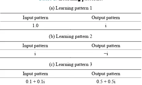
In the experiments, the three sets of (complex-valued) learning patterns shown in Table 1 were used, and the learning constant ε was 0.5. We chose the three-layered 1-1-1 complex-valued neural network where w1=0 and

1 0

ν = were singular points, and the three-layered 2-1-2 real-valued neural network where w =0 and ν=0 were singular points described in Section 4. The comparison using those neural networks is fair because the numbers of the parameters (weights and thresholds) are almost the same: the number of parameters for the 1-1-1 complex- valued network is 8, and that for the 2-1-2 real-valued neural network 7 where a complex-valued parameter

i

[image:4.595.308.539.93.231.2]

z x y= + is counted as two because it consists of a real part x and an imaginary part y. In the real-valued neural network, the real component of a complex number was input into the first input neuron, and the imaginary

Table 1. Learning patterns.

(a) Learning pattern 1

Input pattern Output pattern

1.0 i

(b) Learning pattern 2

Input pattern Output pattern

i −i

(c) Learning pattern 3

Input pattern Output pattern 0.1 + 0.1i 0.5 + 0.5i

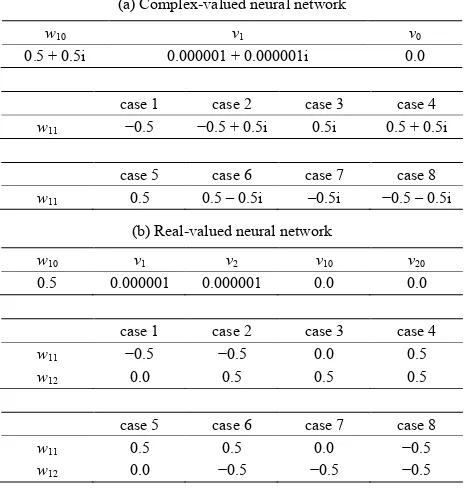
component was input into the second input neuron; the output from the first output neuron was interpreted to be the real component of a complex number, and the output from the second output neuron was interpreted to be the imaginary component. The initial values of the weights and the thresholds were set as shown in Table 2. Note that the initial values of the weights between the hidden layer and the output layer were set in the neighborhood of the singular points: ν =1 0.000001 0.000001i+ in the complex-valued neural network, and

1 0.000001, 2 0.000001

ν = ν = in the real-valued neural

network. The eight initial values (eight cases) were used for the weights w11 or

(

w w11, 12

)

between the input layer and the hidden layer. We judged that learning fi-nished, when the training error was equal to 0.0001, that is, ( )1

(

( )1

)

1; 0.0001

y f− x θ = in the case of the com-plex-valued neural network, and y−g

(

x;θ

)

=0.0001 in the case of the real-valued neural network.

We investigated the learning speed (i.e., learning cycles needed to converge) for each of the 3 learning patterns in the experiments described above. The results of the ex-periments are shown in Table 3. We can find from these experiments that the average learning speed of the com-plex-valued neural network is approximately 1.4 times faster than that of the real-valued neural network. The superscript * of a number means that the weights be-tween the hidden layer and the output layer stayed in the neighborhood of the singular point 0 or

( )

0,0 from the beginning to the end of leaning. Table 4 shows the Euclidean distances between the weights (between the hidden layer and the output layer) and the singular point

0 or

( )

0,0 after the first learning cycle. In every case, the weights of the complex-valued neural network moved in the distance from the singular point 0 compared with those of the real-valued neural network. We believe that this phenomenon originates in the linear combinations of ϕ in Equations (22) and (23) shown in Section 4.

(5)

[image:5.595.56.289.104.348.2]

Table 2. Initial values of the weights and the thresholds.

(a) Complex-valued neural network

w10 v1 v0

0.5 + 0.5i 0.000001 + 0.000001i 0.0 case 1 case 2 case 3 case 4

w11 −0.5 −0.5 + 0.5i 0.5i 0.5 + 0.5i

case 5 case 6 case 7 case 8

w11 0.5 0.5 – 0.5i –0.5i −0.5 – 0.5i

(b) Real-valued neural network

w10 v1 v2 v10 v20

0.5 0.000001 0.000001 0.0 0.0 case 1 case 2 case 3 case 4

w11 −0.5 −0.5 0.0 0.5

w12 0.0 0.5 0.5 0.5

case 5 case 6 case 7 case 8

w11 0.5 0.5 0.0 −0.5

[image:5.595.57.289.436.736.2]

w12 0.0 −0.5 −0.5 −0.5

Table 3. Learning speed (the number of learning cycles needed to converge). Case number means the initial values of the weights between the input layer and the hidden layer (See Table 2). The superscript * of a number means that the weights between the hidden layer and the output layer stayed in the neighborhood of the singlar point 0 or (0, 0) from the beginning to the end of leaning.

Case number 1 2 3 4 5 6 7 8 Complex NN 7 5 3 4 3 5 7 13*

Real NN 13*₁₃* ₇ ₅ ₅ ₅ ₇ ₁₃*

Case number Average Average except the cases*

Complex NN 5.9 4.9

Real NN 8.5 5.8

(b) Learning pattern 2

Case number 1 2 3 4 5 6 7 8 Complex NN 7 13* ₇ ₅ ₃ ₄ ₃ ₅

Real NN 7 5 5 5 7 13*₁₃*₁₃*

Complex NN 5.9 4.9

Real NN 8.5 5.8

(c) Learning pattern 3

Case number 1 2 3 4 5 6 7 8 Complex NN 7 7 6 5 5 5 6 7 Real NN 9 8 8 8 8 8 9 9

Complex NN 6.0 6.0

Real NN 8.4 8.4

Table 4. The Euclidean distances between the weights (be- tween the hidden layer and the output layer) and the sin- gular point 0 or (0, 0) after the first learning cycle: ν1 for

the complex-valued network, and ν for the real-valued neural network. Case number means the initial values of the weights between the input layer and the hidden layer (See Table 2).

Case number 1 2 3 4 5

Complex NN 0.23 0.38 0.44 0.53 0.44 Real NN 0.00 0.00 0.23 0.38 0.38 Case number 6 7 8 Average Complex NN 0.38 0.23 0.00 0.33

Real NN 0.38 0.23 0.00 0.20 (b) Learning pattern 2

Real NN 0.00 0.00 0.00 0.20 (c) Learning pattern 3

Real NN 0.16 0.14 0.13 0.16

weights between the hidden layer and the output layer could not move away from the singular point, but, as a result, the learning speed became slow. And also, the number of cases *_{of the complex-valued neural network} was 1, and that of the real-valued neural network 3, which suggested that the complex-valued neural network was not influenced by singular points compared with the real-valued neural network.

(6)

[image:6.595.70.270.80.239.2]

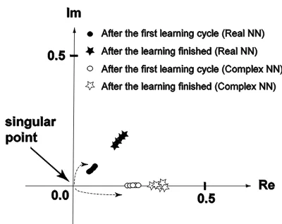
Figure 1. The behavior of the weights between the hidden layer and the output layer. Their initial values were set in the neighborhood of the singular point (the origin). The eight initial values (eight cases) were used for the weights between the input layer and the hidden layer (see Table 2). The distance of the weight of the complex-valued neural network from the singularity after the first learning cycle was larger than that of the real-valued neural network.

6. Conclusions

We compared theoretically and experimentally the in-fluence of the singular points on the learning dynamics in the complex-valued neural network with that in the real- valued neural network. As a result, we found that the linear combination structure in the updating rule of the complex-valued neural network increased the speed of moving away from the singular points; the complex-valued neural network could not be easily influenced by the singular points. This is considered to be a result which supports the fast convergence of the Complex-BP algo-rithm.

It might be premature to conclude the statements de-scribed above are true because this paper deals with only very simple cases such as the network structures and the learning patterns. In the future, we will investigate more complicated cases.

Acknowledgements

The author extends special thanks to the anonymous re-viewers for valuable comments.

REFERENCES

[1] A. Hirose, Ed., “Complex-Valued Neural Networks,” World Scientific Publishing, Singapore, 2003.

[2] T. Nitta, Ed., “Complex-Valued Neural Networks: Uti- lizing High-Dimensional Parameters,” Information Science

Reference, Pennsylvania, 2009.

http://dx.doi.org/10.4018/978-1-60566-214-5

[3] T. Nitta and T. Furuya, “A Complex Back-Propagation Learning,” Transactions of Information Proceedings of

the Society of Japan, Vol. 32, No. 10, 1991, pp. 1319-

1329.

[4] T. Nitta, “A Complex Numbered Version of the Back- Propagation Algorithm,” Proceedings of the World Con- gress on Neural Networks, Portland, Vol. 3, 1993, pp. 576-579.

[5] T. Nitta, “An Extension of the Back-Propagation Algo- rithm to Complex Numbers,” Neural Networks, Vol. 10, No. 8, 1997, pp. 1392-1415.

http://dx.doi.org/10.1016/S0893-6080(97)00036-1 [6] T. Nitta, “Orthogonality of Decision Boundaries in Com-

plex-Valued Neural Networks,” Neural Computation, Vol. 16, No. 1, 2004, pp. 73-97.

http://dx.doi.org/10.1162/08997660460734001

[7] T. Nitta, “Complex-Valued Neural Network and Com- plex-Valued Back-Propagation Learning Algorithm,” In: P. W. Hawkes, Ed., Advances in Imaging and Electron

Physics, Elsevier, Amsterdam, Vol. 152, 2008, pp. 153-

221.

[8] D. E. Rumelhart, etal., “Parallel Distributed Processing,” Vol. 1, MIT Press, 1986.

[9] N. Benvenuto and F. Piazza, “On the Complex Backpro- pagation Algorithm,” IEEE Transactions on Signal Pro-

cessing, Vol. 40, No. 4, 1992, pp. 967-969.

http://dx.doi.org/10.1109/78.127967

[10] G. M. Georgiou and C. Koutsougeras, “Complex Domain Backpropagation,” IEEE Transactions on Circuits and

Systems—II: Analog and Digital Signal Processing, Vol.

39, No. 5, 1992, pp. 330-334.

[11] M. S. Kim and C. C. Guest, “Modification of Backpro- pagation Networks for Complex-Valued Signal Processing in Frequency Domain,” Proceedings of the International

Joint Conference on Neural Networks, Vol. 3, 1990, pp.

27-31.

[12] S. Amari, H. Park and T. Ozekii, “Singularities Affect Dynamics of Learning in Neuromanifolds,” Neural Com-

putation, Vol. 18, No. 5, 2006, pp. 1007-1065.

http://dx.doi.org/10.1162/neco.2006.18.5.1007

[13] F. Cousseau, T. Ozeki and S. Amari, “Dynamics of Learn- ing in Multilayer Perceptrons near Singularities,” IEEE

Transactions on Neural Networks, Vol. 19, No. 8, 2008,

pp. 1313-1328.

http://dx.doi.org/10.1109/TNN.2008.2000391

[14] T. Nitta, “Local Minima in Hierarchical Structures of Complex-Valued Neural Networks,” Neural Networks, Vol. 43, 2013, pp. 1-7.

http://dx.doi.org/10.1016/j.neunet.2013.02.002

[15] H. Wei, J. Zhang, F. Cousseau, T. Ozeki and S. Amari, “Dynamics of Learning near Singularities in Layered Net- works,” Neural Computation, Vol. 20, 2008, pp. 813-843. http://dx.doi.org/10.1162/neco.2007.12-06-414

[16] F. M. De Azevedo, S. S. Travessa and F. I. M. Argoud, “The Investigation of Complex Neural Network on Epi- leptiform Pattern Classification,” Proceedings of the 3rd European Medical and Biological Engineering Confe-