Design and Implementation of 2-Axis Circular
Interpolation Controller in Field Programmable Gate
Array (FPGA) for Computer Numerical Control (CNC)
Machines and Robotics
Mufaddal A. Saifee
Institute of Technology, Nirma University, Ahmedabad, Gujarat,
India - 382481
Usha S. Mehta,
Ph.D.Institute of Technology, Nirma University, Ahmedabad, Gujarat,
India - 382481
ABSTRACT
This paper presents design and implementation of a 2 axis Circular Interpolation Controller in a Xilinx Spartan 6 FPGA to control a 2D Circular motion of a CNC machine or robotic arm. It is implemented using Verilog HDL. Circular motion like linear motion is one of the fundamental movement and an absolute necessity for any motion controller. High precision, repeatability and direction-independent are the three important factors to evaluate the performance of circular interpolation algorithm. To achieve this, a novel analogy Digital Differential Analyzer (DDA) algorithm based circular interpolation controller is implemented, which avoids complex on-the-motion computation with skillful combination of the accumulator and multiplier based hardware structure of FPGA. Hence the real-time performance and precision are enormously improved. The principle of algorithm and its hardware implementation with macro and micro architecture design are discussed in detail in the paper. The simulation results verify the excellent performance and effectiveness of implemented circular interpolation controller.
General Terms
CNC machines, Robotics, Circular interpolation, Motion Controllers, FPGA
Keywords
CNC, Circular interpolation, DDA, Motion Controllers, FPGA, UART
1.
INTRODUCTION
The Heart of Industrial Automation Devices like CNC Machines, Assembly Machines and Robotic Arms are Motion Controllers. Motion controllers control the motion in a predetermined direction through motors. The circular motion of the motor is translated to the robotic arm or CNC tool linearly in small steps. A motor each is required for motion in one particular axis. The controlled motion (line/arc) along the required path trajectory is achieved through various interpolation algorithms run in 2D or 3D space, which are responsible for providing varying rate of pulses to corresponding axis. Therefore, for a 2D motion, the arm or tool is controlled by providing varying rate of pulses to each of the two motors, corresponding to an axis.
Interpolation algorithms are classified as software and hardware interpolation algorithms. Software algorithms are run by processors or controllers serially through instructions, while hardware algorithms are run by dedicated hardware
blocks. Most of the interpolation algorithm uses complex parametric function like sine and cosine for necessary calculations. Software implementation of such algorithms by serial pipelined processors is time consuming and as well as difficult and impractical for real time applications. Thus the efficient, real time complex computation approach is only feasible with hardware logic circuits like FPGA or ASIC having parallel and lower power processing architectures. As compared to ASIC, FPGA’s have lower time to market and simpler design cycle making it an excellent solution for the implementation of motion controllers.
Circular motion controller is the fundamental part of any motion controller. For a 2D circular movement, Circular interpolation controller, controls 2 motors by driving each of them with varying angular velocities and directions depending on the quadrant of motion, to achieve a circular movement from start to end coordinates. Circular motion is approximated by series of small steps. Most of the algorithms of circular interpolation use parametric functions of sine and cosine to perform the necessary calculations. Parametric functions require high degree of numeric precision and consume more hardware and time to be useful in a real-time application. Digital Differential Analyzer (DDA) requires no parametric functions and complex mathematical calculation, so it is fast enough to be used in real-time applications for motion controllers. This paper implements algorithm based on DDA principle [1]. The paper is organized as follows: Section 2
describes the algorithm. Section 3 describes its
implementation. Synthesis and simulation results are given Section 4 and Conclusions are detailed in Section 5.
2.
CIRCULAR INTERPOLATION
ALGORITHM
2.1
Principle of DDA
A random function profile x = f (t) in a rectangular coordinate plane is shown in figure 1.
The area under the curve between T0 to T1 for the function f(t) can be calculated with equation 1.
Fig 1: Area Calculation with DDA
The time between T1 and T0 is divided into small time unit delta(∆)t such that the sum of m unit ∆t equals to T1 - To. Then the area between T1 and T0 is equal to the integration of m time ∆t areas from T0 to T1. Digital differential analyzer comprises an arithmetic unit to perform an integration operation.
If ∆t tends to zero the integration can be approximated with summation of m rectangle showed by the shadowed section in figure 1, so equation 1 becomes.
S = Xi ∆t = ∆t
m−1
i=0
Xi
m−1
i=0
(2)
In equation 2, the parameters satisfy the following requirements.
m ∆t = T1 – T0;
X0 = f(T0) ;
Xm = f(T1)
The complex integration operation is thus decomposed into two fundamental operation, accumulation and multiplication, which can be implemented easily in hardware. Smaller the ∆t, more is the accuracy of the results.
2.2
DDA Circular Interpolation
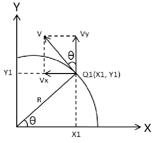
Circular interpolation is far more difficult than the integration operation for curve. To make it clear consider a circular motion in anti-clockwise direction in 1st quadrant as shown in figure 2, where vector V is the angular speed of circular motion. The direction of the speed is the tangent to a circle.
Fig 2: Principal of DDA Circular Interpolation
Let us consider Qi(Xi,Yi) a random point on circle. From the geometrical relation, the following equation can be deduced.
V R=
Vy Xi =
Vx
Yi = k
(3)
The instantaneous displacement at point Qi for each axis in a very small time period ∆ is:
∆y = Vy ∆t = k Xi ∆t (4) ∆x = -Vx ∆t = -k Yi ∆t (5)
[image:2.595.90.247.572.713.2]The sign of displacement depends on the quadrant the track point is in. Taking the absolute displacement of equations 4 and 5.
|∆y| = k |Xi| ∆t (6)
|∆x| = k |Yi| ∆t (7)
From the equation 6, 7, it can be concluded that when the radius of interpolation circle is fixed, the accumulation value for XY displacement only have X coordinate or Y coordinate one variable for the time unit ∆t which is a fixed value. Moreover for one point on circle the speed of X axis is in direct proportion to Y coordinate of this point and vice versa.
From the equation 4 and 5, it can be concluded that if one step is moved in either X or Y direction, the new error result is equal to the previous error result plus a constant value which depends upon the end points of the line in XY coordinates.
2.3
Circular Interpolation Algorithm
For an arc in a 2D plane, two motors are required to control the XY movements of the arc. Since motors move in discrete steps, the actual curve is approximated by a series of small XY motions. The proposed circular interpolation module has 9 only writable registers which are listed in table 1. Through setting values for the registers, several needed parameters, such as the XY coordinates of start and finish point of the arc, arc radius, displacement coefficients in X and Y directions, feed rate and control register are assigned.
Table 1. Registers
Name Addr
-ess
Function
Control 0 Control Register
Feedrate 1 Feedrate of principal axis
motor in revolution/sec
Start_X 2 Start coordinate X direction
Start_Y 3 Start coordinate Y direction
Finish_X 4 Final coordinate X direction
Finish_Y 5 Final coordinate Y direction
Radius 6 Radius of circular arc
Displacement coefficient X
7 Step linear movement in X
direction corresponding to each revolution
Displacement coefficient Y
8 Step linear movement in Y
direction corresponding to each revolution
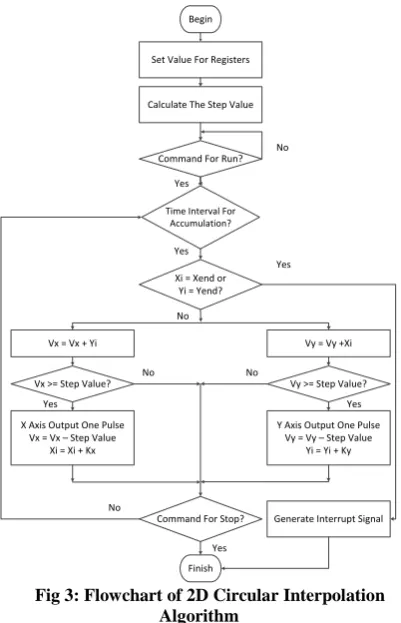
value of Y axis reach to or exceed its upper limit value (unit step displacement of Y axis stepping motor), Yi will add ky.
Begin
Finish Set Value For Registers
Generate Interrupt Signal Command For Run?
Time Interval For Accumulation?
Xi = Xend or Yi = Yend?
Vy >= Step Value? Vx >= Step Value?
Command For Stop?
Vy = Vy +Xi
Y Axis Output One Pulse Vy = Vy – Step Value
Yi = Yi + Ky X Axis Output One Pulse
Vx = Vx – Step Value Xi = Xi + Kx Vx = Vx + Yi
Calculate The Step Value
Yes Yes
Yes
No
Yes
Yes Yes
No No
No
[image:3.595.67.268.97.409.2]No
Fig 3: Flowchart of 2D Circular Interpolation Algorithm
The value of kx, and ky with different situation is listed in table 2.
Table 2. Kx and Ky Values in Different Scenarios
Direction Clockwise Anti-clockwise
Quadrant 1st 2nd 3rd 4th 1st 2nd 3rd 4th
Kx 1 -1 1 -1 -1 1 -1 1
Ky -1 1 -1 1 1 -1 1 -1
The coefficient k and ∆t are constant value. Moreover increment of instantaneous displacement in X direction of the track point depends on Y coordinate end value and vice versa. Therefore XY speed relationship on different points on the circle relates to their XY end coordinates.
As shown in figure 2, the interpolation speed V pps has two speed components, Vx speed in X axis direction and Vy speed in Y axis direction. Vy is the greatest and equal to V, when the track point is on the X axis, that is the frequency of out pluses of Y axis is equal to V pps. So at this point, the accumulating result of accumulator of Y axis is just the upper limit value for one unit step of stepping motor in Y axis, so upper limit value stepvalue can be calculated in following equation.
Stepvalue = 1/V ∆t ∗ R =
Fosc/V Fosc ∗ ∆t∗ R
Having this value the circular interpolation algorithm avoids complex on the motion computation and reduces it to accumulation of the coordinate values. This increases the real-time performance drastically. Because of concurrent processing of FPGA and DDA algorithm the circular
interpolation module reduces the on-the motion computation and has better real-time performance than the other software interpolation.
3.
IMPLEMENTATION
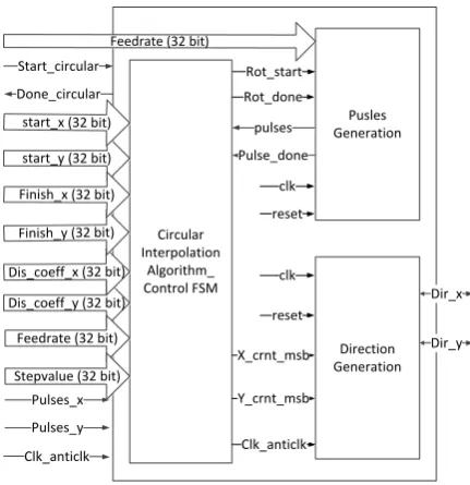
Block diagram of the Circular Interpolation module is shown below in figure 4. It has 6 main modules.
3.1
Buf Dcm Sync Reset (Buffer, Digital
Clock Manager and Synchronous Reset)
This module does the buffering and differential to single ended and frequency down conversion of input clk. It also does the Asynchronous to Synchronous reset conversion to be used as synchronous reset for entire design.3.2
UART
UART is used for asynchronous serial data communication with the Interpolation module. It’s a generic UART supporting all baud rates. The corresponding design uses the 115200 baud rate. UART architecture is based on Recursive Running Sum Filter which provides better noise performance [2].
3.3
UART Register Interface
UART Register Interface is responsible for configuring the Circular Interpolation module. It provides the glue logic between UART and the configuring part. It configures 4, 32 bit registers, namely Control, feedrate, displacement coefficient X and displacement coefficient Y, used for controlling the Circular Interpolation design. Registers function are given in table 1. It also writes the 32 bit coordinates of start and finish of the X and Y axes and radius of each circular interpolation in a 32 bit x 64 block ram.
3.4
RAM
Ram used is a 32 bit wide and 64 deep synchronous simple dual port block ram of FPGA. It is used to hold coordinates of the 2d axis in bunch of five one after other, capable of storing 12 such coordinates. Coordinates are written in RAM by UART Register Interface through UART, while read by Top Control logic.
3.5
Top Control
[image:3.595.56.288.458.507.2]Pulses_X Pulses_Y Dir_X Dir_Y d o n e_ ci rc u la r Start_inst reset Set_ri_out Set_ti_out RX Clk Buf_dcm_sy nc_reset rst Clk200_n Clk200_p Sbuf_out UART UART_reg_interface Sbuf_in TX Sc o n _i n = 8 'h 1 0 Sa m p le s_ b it _i n = 1 6 'h 0 0 8 6 RAM D in a wea Top_control Circular_interpolation_ Control and Algorithm Addra Douta Cntrl Dis_coeff_x Dis_coeff_y feedrate m u l_en d _x m u l_en d _y m u l_ st _y Pulses_ generation Rot_start Cnthf_period Rot_done TX Direction_ Generation Y_crnt_msb X_crnt_msbClk_anticlk Radius Pulse_done Pulse reset clk reset clk reset Clk reset Clk reset Clk reset Clk m u l_ st _x d is _c o ef _m u l_ y d is _c o ef _m u l_ x s te p va lu e C lk _a n ti cl k St ar t ci rc u la r
Fig.4 Block Diagram of Circular Interpolation module
This module calculates the stepvalue and coordinates value according to the accuracy required in millimeters. Stepvalue is calculated from the below formula
Stepvalue = (((fosc / V) / fosc * ∆t)
Where for this implementation, fosc = 50MHz, V = 10000
pulse/rev x 20 rev/s = 0.2 M pulse/sec, ∆t = 20 ns) x 10000 (multiply by 10000 as per the accuracy)
3.6
Circular Interpolation Control and
Algorithm
The DDA principle is used to implement 2D Circular Interpolation algorithm. Top control module provides the movements required in the respective axes. After calculating its algorithm parameters it activates the pulse generation module which provides continuous pulses while direction module gives the direction of rotation. This module compares the current coordinates with the final end coordinates of the arc; if they are not same the velocity vector of the coordinate which is less than the final value is incremented with the current coordinates of the other axes. After incrementing, velocity vector of individual axes is compared to the less than the step value, if it’s so, the corresponding axes coordinates is incremented by its displacement coefficient and velocity vector is decremented by its step value. Moreover the pulse from the pulse generation module is given to the corresponding axes for which the above equality has been less. The above process is repeated until the coordinates reaches their final values forming a circular arc. Pulse
generation module is disabled and above process is repeated for next set of coordinates.
This module, figure 5 is made of three sub modules 1) Circular interpolation algorithm & control FSM, 2) Pulses generation and 3) Direction generation.
Pusles Generation Circular Interpolation Algorithm_ Control FSM Dis_coeff_y (32 bit)
Dis_coeff_x (32 bit) Finish_y (32 bit)
Feedrate (32 bit)
Direction Generation Start_circular
start_y (32 bit) start_x (32 bit)
Feedrate (32 bit)
Pulses_x
Pulses_y
Dir_x
Dir_y Done_circular
Stepvalue (32 bit)
Clk_anticlk clk reset X_crnt_msb Y_crnt_msb Clk_anticlk clk reset Rot_start Rot_done pulses Pulse_done
Finish_x (32 bit)
[image:4.595.318.534.510.733.2]3.6.1
Circular interpolation algorithm and
control FSM
The inputs to this module are absolute displacement coordinates of start and end points and the displacement coefficient for the respective x and y axis. Feed rate is given directly to pulses generation module. It also calculates the unsigned value of the current coordinates required to increment the velocity vectors of x and y axis. It calculates the signed displacement coefficient values from the unsigned displacement coefficient depending on the quadrant the circulating point is and the direction of circular interpolation.
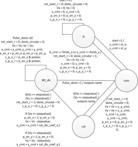
This module performs the interpolation algorithm described in introduction section. It controls the pulse generation module, and pulses generated by it are given to one of the axis or both depending on the corresponding axis velocity vector value is greater than the stepvalue. Heart of this module is its control FSM, figure 6. This FSM has four states 1) st, 2) com 3) cal and 4) wt_dn.
start = 0 / rot_start_r = 0; done_circular = 0;
Vx = 0; Vy = 0; x_crnt = 0; y_crnt = 0; p_en_x = 0; p_en_y = 0; s_p_x_r = 0; s_p_y_r = 0;
X_crnt == finish_x or y_crnt == finish_y / rot_start_r = 0; done_circular = 1;
Vx = 0; Vy = 0; x_crnt = 0; y_crnt = 0; p_en_x = 0; p_en_y = 0; s_p_x_r = 0; s_p_y_r = 0;
start =1 / x_crnt = st_x; y_crnt = st_y;
Pulse_done =1 / outputs same
!((Vx >= stepvalue) | (Vy >= stepvalue)) / rot_start_r = 1; done_circular = 0;
s_p_x_r = 0; s_p_y_r = 0; If (Vx >= stepvalue){ p_en_x = 1; p_en_y = 0;
Vx = Vx - stepvalue; x_crnt = x_crnt + cal_dis_coef_x;}
If (Vy >= stepvalue){ p_en_y = 1; p_en_x = 0;
Vy = Vy - stepvalue; y_crnt = y_crnt + cal_dis_coef_y;}
!((Vx >= stepvalue) | (Vy >= stepvalue)) /
outputs same done_circular = 0;/ rot_start_r = 0; Vx = Vx + u_y_crnt; Vy = Vy + u_x_crnt; x_crnt = x_crnt;
y_crnt = y_crnt; p_en_x = 0; p_en_y = 0;
s_p_x_r = 0; s_p_y_r = 0; cal
com st
Wt_dn Pulse_done =0/ rot_start_r = 0; done_circular = 0;
Vx = Vx; Vy = Vy; x_crnt = x_crnt; y_crnt = y_crnt; p_en_x = p_en_x; p_en_y = p_en_y;
[image:5.595.57.290.278.526.2]s_p_x_r = p_en_x & pulses; s_p_y_r = p_en_y & pulses;
Fig 6: Circular Interpolation Algorithm FSM
St (Start): In St state, until start equal to 1 is detected, all
outputs, enable and pulses signals for two axis, velocity vectors and current coordinates of two axes, start and stop interpolation signals are all 0. When start is 1 FSM jumps to Com state.
Com (Compare): In this state if actual coordinates of either x
or y axis becomes equal to their final arc end points then FSM jumps to St state resetting all its output and raising circulation done (done_circular) to 1, indicating the interpolation algorithm is complete for the current coordinate values. If it’s not equal, it increments the respective x and y coordinates velocity vector with the unsigned value of the current y and x coordinates value and jumps to Cal state.
Cal (Calculation): If either of the axis velocity vector is
greater than or equal to the stepvalue than FSM jumps to wait state. If velocity vector of x axis is greater than the stepvalue than it is decremented by the step value, x axis current coordinate is incremented by its signed displacement coefficient and x axis pulse enable is made 1. Similarly is done for y axis. If neither of the axis velocity vector is greater
than or equal to the stepvalue than FSM jumps to com state without changing the outputs.
Wt_dn (Wait done): In this state FSM waits for the pulse
done signal from pulse generator. When it is detected it moves to Com state for further interpolation calculation. While it is in this state all output values are preserved, while pulse outputs to respective axes are given out by anding their respective enable pulses with the pulse generated from pulse generator module.
3.6.2
Pulse Generation module
Pulse generation module is responsible for generating pulses to servo drive of both the axis depending on the input feedrate. Pulse Generation Module starts generating pulses on detection of Rotation start (rot_start) and stops generating pulses on getting Rotation done signal (rot_done) from Circular Interpolation Control and Algorithm Module. Its heart is control FSM which generates pulses and pulse_done signal. Pulses generated have 50% duty cycle. Its control FSM, figure 7 has 3 states 1) Idle, 2) pos_half and 3) neg_half.
Cnt_equal = 1 / cnt_en = 0 Cnt_equal = 0 /
cnt_en = 1, pulse = 0
Cnt_equal = 1 && rot_done = 1/
cnt_en = 0, pulse_done = 1
Neg_half Pos_half
idle
Cnt_equal = 1 / cnt_en = 0, pulse_done = 1
Cnt_equal = 0 / cnt_en = 1,
pulse = 1 Rot_start =1 rot_start = 0 /
cnt_en = 0, pulse = 0, pulse_done =
0
Fig 7: Pulse Generation FSM
Idle: FSM remains in this state until it gets rotation start
(rot_start) signal, after which it jumps to pos_half state.
Pos_half:(Positive half cycle) In this state pulses signal
remains high for cnt_hf_period. Cnt_hf_period is the half of the period configured in the feed rate. A count enable (cnt_en) is made 1 which causes the counter to count up to cnt_hf_period. The comparator output equals 1 when counter value equals to cnt_hf_period. This causes FSM to jump to Neg_half state. cnt_en is made 0.
Neg_half:(Negetive half cycle) In this state pulses signal
remains low for cnt_hf_period. If counter reaches cnt_hf_period and rotation done (rot_done) signal is also 1, indicating circular interpolation for the given coordinate is completed the FSM moves to idle state. While if counter comparator output is equal to 1 and rotation done signal is not 1, FSM jumps to Pos_half state. In above both conditions cnt_en is made 0 and pulse done is raised high.
3.6.3
Direction Generation
[image:5.595.324.537.302.489.2]Table 3. Direction Determination
X current
MSB
Y current
MSB
Clock/ Anti-clock
Quad Directi
on X
Directi on Y
0 0 0 1st 1 0
0 0 1 1st 0 1
0 1 0 4th 0 0
0 1 1 4th 1 1
1 0 0 2nd 1 1
1 0 1 2nd 0 0
1 1 0 3rd 0 1
1 1 1 3rd 1 0
4.
RESULTS
4.1
Synthesis Results
[image:6.595.313.561.96.312.2]Selected Spartan 6 FPGA Device: 6slx45tfgg484-3
Table 4. Device Utilization Summary
Type of Resource Utilization
Number
Utilization Percentage
No. of Slice Registers 1102 out of
54576
1%
No. of Slice LUTs 1871 out of
27288
6%
No. of Slice LUTs used as Logic
1871 out of 27288
6%
No. of bonded IOBs 13 out of 296 4%
No. of Block RAM/FIFO 1 out of 116 0%
No. of BUFG/BUFGCTRLs
2 out of 16 12%
No. of DSP48A1s 12 out of 58 20%
Device utilization summary shows that the implemented algorithm is highly hardware efficient consuming only 1871, 6 input LUTs and 1102 flip flops.
[image:6.595.54.287.272.414.2]4.2
Simulation Results
Figure 8 Waveform1 shows that all parameters are configured through UART. Absolute addressing is used for coordinates. The address and data lines logic of the RAM are shown. Coordinates are fetched from the RAM and updated to start x, start y, finish x, finish y and radius. Stepvalue calculated, start circular interpolation signals and rest control signals are also visible.
Fig 8: Waveform1
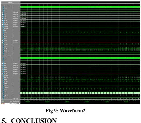
In Waveform 2, figure 9 the circular interpolation algorithm and its FSM signals are shown.
Fig 9: Waveform2
5.
CONCLUSION
This paper explains detail design and implementation of 2 axis circular interpolation module. It gives brief explanation of DDA based circular interpolation algorithm, explains it macro and micro level architecture design and shows its simulation results. DDA algorithm and concurrent hardware processing of FPGA helps the circular interpolation controller to achieve excellent real time performance. Simulation results show the precision and performance to be excellent. Synthesis report also shows it to be hardware efficient by consuming fewer Flip flops and LUTS. Excellent real time operation, good precision and optimum hardware resources makes the FPGA-based circular interpolation controller have excellent performance and useful for any motion controller for CNC machines and Robotic arms.
6.
REFERENCES
[1] Weihai Chen, Zhaojin Wen, ZhiyueXu and Jingmeng
Liu, “Implementation of 2-axis Circular Interpolation for a FPGA-based 4-axis Motion Controller” IEEE International Conference on Control and Automation, 2007, pp. 600-605
[2] Himanshu Patel, Sanjay Trivedi, R. Neelkanthan, V. R.
Gujraty, “A Robust UART Architecture Based on Recursive Running Sum Filter for Better Noise Performance” Conference Proceedings: 20th VLSI Design - 6th Embedded Systems, The Institute of Electrical and Electronics Engineers, Inc. January 2007,
pp 819-823.
[3] Mufaddal A. Saifee and Dr. Usha S. Mehta, “Design and
Implementation of 3 Axis Linear Interpolation Controller in FPGA for CNC Machines and Robotics” International Journal of Advanced Research in Engineering and Technology, Volume 5, Issue 9, Sept 2014, pp. 52-62
[4] K Goldberg, and M Goldberg, “XY interpolation
algorithms”, Robotics Age, No 5, May 1983, pp.104-105
[5] K Goldberg, and M Goldberg, “XY interpolation
algorithms”, Robotics Age, No 5, May 1983, pp.104-105
[6] Z. Zhang, C. W. Peng, and L. G. Yin, “Motion Controller
[image:6.595.55.310.547.730.2][7] J. L. Liu, W. Liu, and C. Y. Yu, “Complete Numeric CNC System and Its Kernel Chip MCX314”, Electronic Design & Application World,no.8, 2004, pp.104-106
[8] P. Q. Yue, and J. S. Wang "Motion Controller IC MCX3
14 and Numerical Control System Design". Beijing: Beihang University Press Nov.2002
[9] X. Qing, C .D. Zhou and W. Wang "Hardware Design of
Arc Interpolator Based on FPGA", Lathe and Fluid Power, No 5, 20026,pp.104-105
[10]Jung Uk Cho, Quy Ngoc Le, and Jae Wook Jeon, “An
FPGA-Based Multiple-Axis Motion Control Chip” IEEE Transactions on Industrial Electronics Vol. 56, No. 3, Mar. 2009
[11]B. T. Zhou, and B. J. Wang "A DDA arc interpolator for
digital differential analyzer based on FPGA ", Electric Drive Automation. Vol.27, No .5, 2005, pp. 16-18
[12]S. L. Yang "The quick algorithm and realization of DDA