Condensed Matrix Descriptor for Protein Sequence Comparison

(1)

http://dx.doi.org/10.4236/ijamsc.2016.41001

Condensed Matrix Descriptor for Protein

Sequence Comparison

Soumen Ghosh

1

_{, Jayanta Pal}

2

_{, Bansibadan Maji}

3

_{, Dilip Kumar Bhattacharya}

4 1

_{Department of Information Technology, Narula Institute of Technology, Kolkata, India}

2

_{Department of Computer Science & Engineering, Narula Institute of Technology, Kolkata, India}

3

_{Department of Electronics & Communication Engineering, National Institute of Technology, Durgapur, India}

4

_{Department of Pure Mathematics, Calcutta University, Kolkata, India}

Received 21 December 2015; accepted 14 March 2016; published 17 March 2016

Copyright © 2016 by authors and Scientific Research Publishing Inc.

This work is licensed under the Creative Commons Attribution International License (CC BY).

http://creativecommons.org/licenses/by/4.0/

Abstract

The present paper develops a novel way of reducing a protein sequence of any length to a real

symmetric condensed 20 × 20 matrix. This condensed matrix can be nicely applied as a protein

sequence descriptor. In fact, with such a condensed representation, comparison of two protein se-

quences is reduced to a comparison of two such 20 × 20 matrices. As each square matrix has a

unique Alley Index/normalized Alley Index, such index is conveniently used in getting distance

matrix to construct Phylogenetic trees of different protein sequences. Finally protein sequence

comparison is made based on these Phylogenetic trees. In this paper three types viz., NADH

dehy-drogenase subunit 3 (ND3), subunit 4 (ND4) and subunit 5 (ND5) of protein sequences of nine

species, Human, Gorilla, Common Chimpanzee, Pygmy Chimpanzee, Fin Whale, Blue Whale, Rat,

Mouse and Opossum are used for comparison.

Keywords

Amino Acids, Condensed Matrix, Eigen Values, Matrix Invariants, ALE Index

1. Introduction

(2)

pro-tein structure, which are based only on sequence information, started several years ago. Sequence alignment is a

way of arranging the sequences of DNA, RNA, or protein to identify regions of similarity that may be a

conse-quence of functional, structural, or evolutionary relationships between the seconse-quences [1]. Existing methods for

sequence comparison can be classified into alignment based methods and alignment-free methods. Alignment-

based methods use dynamic programming, a regression technique that finds an optimal alignment by assigning

scores to different possible alignments and picking the alignment with the highest score. Dynamic programming

method is an accurate method for comparison of two sequences. There are two types of dynamic programming:

global dynamic programming which is applied for comparing sequences as a whole [2] [3] and local dynamic

programming which is applied to compare selected portions of the sequences [4]. For multiple sequence

align-ments (MSA) there are many methods, some of them are given in [5]-[7]. In parallel there are many algorithms

available for multiple sequence comparison; some of them are listed in [8]-[11]. But the main difficulty in

mul-tiple sequence alignment is the computational complexity. In fact a naïve MSA takes O(l

N

) time for completion

of the program, where N is the number of sequences for comparison, each having a length

l

. Therefore as an

ternative to sequence based alignment, alignment free methods are chosen. Such alignment free methods are

al-ready known for comparison of DNA/RNA sequence comparison [12]-[14]. Alignment free methods are based

on graphical representation, which is obtained from the numerical values given to the nucleotides. Next step is to

obtain the descriptors for obtaining distance matrices. One way is to characterize the graphs by obtaining

direct-ly some invariants like geometrical centres, graph radii, variances etc. [15] and to use these invariants as

de-scriptors to obtain distance matrices for constructing phylogenetic trees of comparison. The other way is to

transform the graphical representation into another mathematical object, a real symmetric matrix. The matrices

may be of L/L, M/M or J/J types [16]. J/J matrix is applicable only for 3D representation. Once a real symmetric

matrix M is obtained, there are different invariants associated with this matrix such as the average matrix

ele-ment, the average row sum, the leading eigen value, Weiner number and the Alley index/normalized Alley index

[17]. These may be used to obtain the distance matrix to obtain phylogenetic trees for comparison of DNA/RNA

sequences. Now protein sequences are to some degree similar to DNA/RNA sequences in the sense that

DNA/RNA sequences contain four nucleotides, whereas protein sequences contain twenty amino acids. Thus the

graphical representation methods for comparison of DNA/RNA may be extended to protein sequences as well.

Currently, many researchers have proposed different methods for the graphical representation of protein

se-quences [18]-[33]. In most of these existing methods, the main drawbacks are that the higher the dimension of

the protein sequence graphs, the heavier the computation complexity of the methods or the lower the recognition

degree of the protein sequence graphs [34] [35]. In the methods proposed in [36]-[38], the main drawbacks are

that the 3D graphics seem to be more complex and have lower visibility than the 2D graphics, and, in addition,

to obtain the sequence invariants from the graphics, complex matrices are required to be constructed, which

need much computation and storage.

Lei Wang, Hui Peng and Jinhua Zheng [39] proposed a novel method for analyzing the similarity/dissimilar-

rity by combining the idea of the sequence alignment and the graphical representation methods to avoid the

weakness of both of these two methods to some degree. Principal components analysis (PCA) is a standard tool

in multivariate data analysis to reduce the number of dimensions, which has been proved to be effective in the

process of protein sequence analysis [40]-[42]. They used 29 different spike proteins, which are widely used as

the test data [25]-[34] [43].

Anyway it is very difficult to make direct comparison of protein sequences owing to their very long sizes and

unequal lengths. Actually a direct comparison between protein sequences would not only be tedious but would

involve steps not yet fully resolved, such as how to proceed when comparing sequences of different lengths. A

possible strategy to avoid such difficulties is to represent the protein sequences by suitable condensed matrices.

In this way, comparison between sequences reduces to comparison between matrices. Similar reduction of DNA

sequence to 4 × 4 matrices is already known [44]. The case was simple in the sense that it was needed to

consid-er representation of four nucleotides only, whconsid-ere as in the case of protein sequence it is much more difficult to

handle twenty amino acids simultaneously. To make the problem manageable, we start with a suitable numerical

representation of the sequence and finally reduce it in the form of a condensed 20 × 20 matrix of unique size.

2. Methods of Constructing 20 × 20 Matrices of Protein Sequences

(3)

acids, so in this case, the final reduction is a 9 × 9 matrix.

2.1. First Step: To Calculate Distance of Each Label from the Neighboring Labels

In the first step we construct “distance” of each label from the neighboring labels of the same and different kind

of amino acid. It is calculated by numbering the amino acids in the protein sequence starting from 0 (zero) for

the first amino acid and starting from 1 (one) for the other amino acids. Thereby we get a 12 × 12 matrix, where

12 is the length of the protein sequence (as shown in Table 2). The entries of the matrix represent frequencies of

occurrences of amino acids.

2.2. Second Step: To Group Together All Similar Amino Acids

Second step involves grouping together all similar amino acids. First of all, the amino acids are taken

alphabeti-cally as D, E, K, L, M, P, R, V, W. Next the bases of the same kind are grouped together. The elements of the

matrix correspond to the serial distance of the first 12 amino acids. The rearranged 12 × 12 matrix is shown in

Table 3.

2.3. Third Step: To Obtain Sub-Matrices

From Table 3, we obtain forty five sub-matrices (DD, DE, DK, DL, DM, DP, DR, DV, DW, EE, EK, EL, EM,

EP, ER, EV, EW, KK, KL, KM, KP, KR, KV, KW, LL, LM, LP, LR, LV, LW, MM, MP, MR, MV, MW, PP,

PR, PV, PW, RR, RV, RW, VV, VW, WW). Some of them are shown in Tables 4-6.

2.4. Fourth Step: To Obtain Final Reduced 9 × 9 Condensed Matrix

All the sub-matrices are not square matrices. So we cannot get Eigen values of all the sub-matrices.

Mathemati-cally it may be shown that the average of all the elements of a square matrix nearly approximates the highest

Eigen value of that matrix. So in the third step we consider the average of all the elements of each sub-matrix

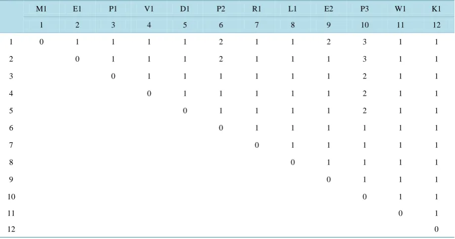
Table 1.

Small sample of protein sequences.

1 2 3 4 5 6 7 8 9 10 11 12

M E P V D P R L E P W K

Table 2.

12 × 12 matrix obtained by considering the 12 amino acids from the beginning of the sequence of

Table 1

.

M1 E1 P1 V1 D1 P2 R1 L1 E2 P3 W1 K1

1 2 3 4 5 6 7 8 9 10 11 12

1 0 1 1 1 1 2 1 1 2 3 1 1

2 0 1 1 1 2 1 1 1 3 1 1

3 0 1 1 1 1 1 1 2 1 1

4 0 1 1 1 1 1 2 1 1

5 0 1 1 1 1 2 1 1

6 0 1 1 1 1 1 1

7 0 1 1 1 1 1

8 0 1 1 1 1

9 0 1 1 1

10 0 1 1

11 0 1

[image:3.595.88.538.485.721.2]

(4)

Table 3.

Rearranged 12 ×12 matrix.

D1 E1 E2 K1 L1 M1 P1 P2 P3 R1 V1 W1

5 2 9 12 8 1 3 6 10 7 4 11

5 0 1 1 1 1 1 1 1 2 1 1 1

2 0 1 1 1 1 1 2 3 1 1 1

9 0 1 1 2 1 1 1 1 1 1

12 0 1 1 1 1 1 1 1 1

8 0 1 1 1 1 1 1 1

1 0 1 2 3 1 1 1

3 0 1 2 1 1 1

6 0 1 1 1 1

10 0 1 1 1

7 0 1 1

4 0 1

11 0

Table 4.

DE sub-matrix.

E1 E2

D1 1 1

Table 5.

EP sub-matrix.

P1 P2 P3

E1 1 2 3

E2 1 1 1

Table 6.

PR sub-matrix.

R1

P1 1

P2 1

P3 1

and finally get the 9 × 9 condensed matrix given in Table 7.

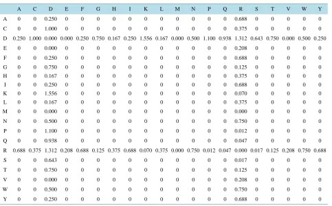
3. Construction of 20 × 20 Condensed Matrix for (HIV 1) Tat Protein

We consider the sequence of Human Immunodeficiency Virus 1 (HIV 1) Tat Protein, which has 86 amino acids.

By following steps one to three as above, we get 86 × 86 rearranged matrix and calculate the sub-matrices Two

such sub-matrices AA and CG are given in Table 8 and Table 9 respectively;

The final 20 × 20 condensed matrix is given in Table 10.

4. Sensitivity of the 20 × 20 Condensed Matrix

Now we change the protein sequence of Human Immunodeficiency Virus 1 a little bit. We interchange the 5th

and 56th amino acid i.e. we take the 5th amino acid as R instead of D and take the 56th amino acid as D instead

of R and we get the following (Table 11).

(5)

Table 7.

9 × 9 Condensed matrix.

D E K L M P R V W

D 0 1 1 1 1 1.33 1 1 1

E 1 0.5 1 1 1.5 1.5 1 1 1

K 1 1 0 1 1 1 1 1 1

L 1 1 1 0 1 1 1 1 1

M 1 1.5 1 1 0 2 1 1 1

P 1.33 1.5 1 1 2 0.89 1 1 1

R 1 1 1 1 1 1 0 1 1

V 1 1 1 1 1 1 1 0 1

W 1 1 1 1 1 1 1 1 0

Table 8.

AA sub-matrix.

AA 21 42

21 0 1

42 1 0

Table 9.

CG sub-matrix.

CG 15 44 48 61 79 83

22 1 1 2 3 4 5

25 2 1 2 3 4 5

27 3 1 2 3 4 5

30 4 1 2 3 4 5

31 5 1 2 3 4 5

34 6 1 2 3 4 5

37 7 1 2 3 4 5

To test for sensitivity, we generate a 20 × 20 matrix, which contains the cell-by-cell differences of the content

of Table 10 and Table 12. This is given in Table 13.

The result shows that our method of constructing the 20 × 20 Condensed Matrix is highly sensitive. Little bit

of change in the sequence of a protein affects the content of the final 20 × 20 condense matrix.

5. Comparison of Protein Sequences

As we have already illustrated how to reduce a protein sequence to a condensed 20 × 20 matrix, so the problem

of comparison of two protein sequences reduces to the problem of comparison of two 20 × 20 matrices. In this

paper we solve this problem by ALE index [17].

ALE index for a matrix M is defined by

( )

1

1 1

1

2

m F

n

M

n

χ χ

=





_

+

−





_





where,

(

)

2 _T

1

, 1 , 1

,

n n

ij ij

m F

i j i j

M

a

M

a

tr M M

= =

(6)

Table 10.

20 × 20 condense matrix of the protein sequence of Human Immunodeficiency Virus 1 (HIV 1) tat protein.

A C D E F G H I K L M N P Q R S T V W Y

A 0.500 2.500 1.250 1.333 1.250 2.750 1.333 1.250 2.611 1.500 1.500 1.000 2.250 3.312 3.688 3.214 2.167 1.333 1.500 1.250

C 2.500 2.286 2.500 3.000 1.429 3.167 2.286 1.500 3.492 2.333 4.000 3.143 3.500 3.893 4.000 3.571 2.952 2.286 4.000 1.857

D 1.250 2.500 0.500 1.333 1.250 2.250 1.500 1.250 3.000 1.500 1.500 1.000 2.900 2.750 2.750 2.500 2.250 1.333 1.000 1.250

E 1.333 3.000 1.333 0.889 1.333 2.667 1.667 1.333 3.667 1.556 2.000 1.000 3.500 3.333 3.083 3.000 2.667 1.556 1.000 1.333

F 1.250 1.429 1.250 1.333 0.500 2.750 1.333 1.500 2.333 1.500 1.500 1.500 2.250 3.312 3.688 3.214 2.167 1.333 1.500 1.250

G 2.750 3.167 2.250 2.667 2.750 1.944 2.500 2.417 2.907 2.500 3.500 2.667 2.933 2.958 3.021 2.833 2.556 2.500 3.500 2.417

H 1.333 2.286 1.500 1.667 1.333 2.500 0.889 1.333 2.667 1.556 2.000 1.333 2.500 3.208 2.875 3.048 2.333 1.556 2.000 1.333

I 1.250 1.500 1.250 1.333 1.500 2.417 1.333 0.500 2.111 1.333 1.500 1.500 2.250 3.000 3.688 3.214 1.917 1.333 1.500 1.250

K 2.611 3.492 3.000 3.667 2.333 2.907 2.667 2.111 2.963 2.778 5.000 3.333 3.778 3.486 3.528 3.206 2.944 2.889 5.000 2.611

L 1.500 2.333 1.500 1.556 1.500 2.500 1.556 1.333 2.778 0.889 2.000 1.333 2.667 2.917 2.875 2.905 2.222 1.556 1.333 1.333

M 1.500 4.000 1.500 2.000 1.500 3.500 2.000 1.500 5.000 2.000 0.000 1.000 5.500 4.500 4.500 4.000 3.500 2.000 1.000 1.500

N 1.000 3.143 1.000 1.000 1.500 2.667 1.333 1.500 3.333 1.333 1.000 0.000 2.000 3.625 3.625 3.143 2.000 1.333 1.000 1.500

P 2.250 3.500 2.900 3.500 2.250 2.933 2.500 2.250 3.778 2.667 5.500 2.000 3.300 3.513 3.600 3.229 2.933 2.867 3.100 2.250

Q 3.312 3.893 2.750 3.333 3.312 2.958 3.208 3.000 3.486 2.917 4.500 3.625 3.513 2.625 3.359 3.036 2.917 2.917 4.500 3.312

R 3.688 4.000 2.750 3.083 3.688 3.021 2.875 3.688 3.528 2.875 4.500 3.625 3.600 3.359 2.625 3.196 3.000 3.083 3.625 3.688

S 3.214 3.571 2.500 3.000 3.214 2.833 3.048 3.214 3.206 2.905 4.000 3.143 3.229 3.036 3.196 2.286 2.786 3.048 4.000 2.857

T 2.167 2.952 2.250 2.667 2.167 2.556 2.333 1.917 2.944 2.222 3.500 2.000 2.933 2.917 3.000 2.786 1.944 2.333 3.500 1.917

V 1.333 2.286 1.333 1.556 1.333 2.500 1.556 1.333 2.889 1.556 2.000 1.333 2.867 2.917 3.083 3.048 2.333 0.889 1.333 1.333

W 1.500 4.000 1.000 1.000 1.500 3.500 2.000 1.500 5.000 1.333 1.000 1.000 3.100 4.500 3.625 4.000 3.500 1.333 0.000 1.500

Y 1.250 1.857 1.250 1.333 1.250 2.417 1.333 1.250 2.611 1.333 1.500 1.500 2.250 3.312 3.688 2.857 1.917 1.333 1.500 0.500

Table 11.

Modified or changed protein sequence of Human Immunodeficiency Virus 1 (HIV 1) tat protein (length 86 amino acids).

MEPVRPRLEPWKHPGSQPKTACTNCYCKKCCFHCQVCFITKALGISYGRKKRRQRDRPPQGSQTHQVSLSKQPTSQSRGDPTGPKE

The ALE-index is very simple for calculation so that it can be directly used to handle long sequences. If

de-sired, one can introduce weighting procedure that will normalize magnitudes of the ALE-indices to reduce

vari-ations caused by comparison of matrices of different sizes. For instance

, one can consider instead of χ a

norma-lized ALE-

index χ' = χ/n, where n is the length of the sequence and the order of the corresponding matrix as

well.

6. Sequences for Comparison

We have used the NADH dehydrogenase subunit 3 (ND3), subunit 4 (ND4) and subunit 5 (ND5) protein

se-quences of nine species for comparison as shown in Table 14.

7. Measures of Comparison of Sequences from Reduced Matrices

(7)

Table 12.

20 × 20 Condense matrix of modified or changed protein sequence of Human Immunodeficiency Virus 1 (HIV 1).

A 0.500 2.500 1.500 1.333 1.250 2.750 1.333 1.250 2.611 1.500 1.500 1.000 2.250 3.312 3.000 3.214 2.167 1.333 1.500 1.250

C 2.500 2.286 1.500 3.000 1.429 3.167 2.286 1.500 3.492 2.333 4.000 3.143 3.500 3.893 3.625 3.571 2.952 2.286 4.000 1.857

D 1.500 1.500 0.500 1.333 1.500 1.500 1.333 1.500 1.444 1.333 1.500 1.500 1.800 1.812 1.438 1.857 1.500 1.333 1.500 1.500

E 1.333 3.000 1.333 0.889 1.333 2.667 1.667 1.333 3.667 1.556 2.000 1.000 3.500 3.333 2.875 3.000 2.667 1.556 1.000 1.333

F 1.250 1.429 1.500 1.333 0.500 2.750 1.333 1.500 2.333 1.500 1.500 1.500 2.250 3.312 3.000 3.214 2.167 1.333 1.500 1.250

G 2.750 3.167 1.500 2.667 2.750 1.944 2.500 2.417 2.907 2.500 3.500 2.667 2.933 2.958 2.896 2.833 2.556 2.500 3.500 2.417

H 1.333 2.286 1.333 1.667 1.333 2.500 0.889 1.333 2.667 1.556 2.000 1.333 2.500 3.208 2.500 3.048 2.333 1.556 2.000 1.333

I 1.250 1.500 1.500 1.333 1.500 2.417 1.333 0.500 2.111 1.333 1.500 1.500 2.250 3.000 3.000 3.214 1.917 1.333 1.500 1.250

K 2.611 3.492 1.444 3.667 2.333 2.907 2.667 2.111 2.963 2.778 5.000 3.333 3.778 3.486 3.458 3.206 2.944 2.889 5.000 2.611

L 1.500 2.333 1.333 1.556 1.500 2.500 1.556 1.333 2.778 0.889 2.000 1.333 2.667 2.917 2.500 2.905 2.222 1.556 1.333 1.333

M 1.500 4.000 1.500 2.000 1.500 3.500 2.000 1.500 5.000 2.000 0.000 1.000 5.500 4.500 4.500 4.000 3.500 2.000 1.000 1.500

N 1.000 3.143 1.500 1.000 1.500 2.667 1.333 1.500 3.333 1.333 1.000 0.000 2.000 3.625 2.875 3.143 2.000 1.333 1.000 1.500

P 2.250 3.500 1.800 3.500 2.250 2.933 2.500 2.250 3.778 2.667 5.500 2.000 3.300 3.513 3.612 3.229 2.933 2.867 3.100 2.250

Q 3.312 3.893 1.812 3.333 3.312 2.958 3.208 3.000 3.486 2.917 4.500 3.625 3.513 2.625 3.406 3.036 2.917 2.917 4.500 3.312

R 3.000 3.625 1.438 2.875 3.000 2.896 2.500 3.000 3.458 2.500 4.500 2.875 3.612 3.406 2.625 3.179 2.875 2.875 2.875 3.000

S 3.214 3.571 1.857 3.000 3.214 2.833 3.048 3.214 3.206 2.905 4.000 3.143 3.229 3.036 3.179 2.286 2.786 3.048 4.000 2.857

T 2.167 2.952 1.500 2.667 2.167 2.556 2.333 1.917 2.944 2.222 3.500 2.000 2.933 2.917 2.875 2.786 1.944 2.333 3.500 1.917

V 1.333 2.286 1.333 1.556 1.333 2.500 1.556 1.333 2.889 1.556 2.000 1.333 2.867 2.917 2.875 3.048 2.333 0.889 1.333 1.333

W 1.500 4.000 1.500 1.000 1.500 3.500 2.000 1.500 5.000 1.333 1.000 1.000 3.100 4.500 2.875 4.000 3.500 1.333 0.000 1.500

[image:7.595.60.544.419.719.2]

Y 1.250 1.857 1.500 1.333 1.250 2.417 1.333 1.250 2.611 1.333 1.500 1.500 2.250 3.312 3.000 2.857 1.917 1.333 1.500 0.500

Table 13.

20 × 20 matrix of the differences of

Table 8

and

Table 10

.

A 0 0 0.250 0 0 0 0 0 0 0 0 0 0 0 0.688 0 0 0 0 0

C 0 0 1.000 0 0 0 0 0 0 0 0 0 0 0 0.375 0 0 0 0 0

D 0.250 1.000 0.000 0.000 0.250 0.750 0.167 0.250 1.556 0.167 0.000 0.500 1.100 0.938 1.312 0.643 0.750 0.000 0.500 0.250

E 0 0 0.000 0 0 0 0 0 0 0 0 0 0 0 0.208 0 0 0 0 0

F 0 0 0.250 0 0 0 0 0 0 0 0 0 0 0 0.688 0 0 0 0 0

G 0 0 0.750 0 0 0 0 0 0 0 0 0 0 0 0.125 0 0 0 0 0

H 0 0 0.167 0 0 0 0 0 0 0 0 0 0 0 0.375 0 0 0 0 0

I 0 0 0.250 0 0 0 0 0 0 0 0 0 0 0 0.688 0 0 0 0 0

K 0 0 1.556 0 0 0 0 0 0 0 0 0 0 0 0.070 0 0 0 0 0

L 0 0 0.167 0 0 0 0 0 0 0 0 0 0 0 0.375 0 0 0 0 0

M 0 0 0.000 0 0 0 0 0 0 0 0 0 0 0 0.000 0 0 0 0 0

N 0 0 0.500 0 0 0 0 0 0 0 0 0 0 0 0.750 0 0 0 0 0

P 0 0 1.100 0 0 0 0 0 0 0 0 0 0 0 0.012 0 0 0 0 0

Q 0 0 0.938 0 0 0 0 0 0 0 0 0 0 0 0.047 0 0 0 0 0

R 0.688 0.375 1.312 0.208 0.688 0.125 0.375 0.688 0.070 0.375 0.000 0.750 0.012 0.047 0.000 0.017 0.125 0.208 0.750 0.688

S 0 0 0.643 0 0 0 0 0 0 0 0 0 0 0 0.017 0 0 0 0 0

T 0 0 0.750 0 0 0 0 0 0 0 0 0 0 0 0.125 0 0 0 0 0

V 0 0 0.000 0 0 0 0 0 0 0 0 0 0 0 0.208 0 0 0 0 0

W 0 0 0.500 0 0 0 0 0 0 0 0 0 0 0 0.750 0 0 0 0 0

(8)

[image:8.595.57.540.101.279.2]

Table 14.

List of nine species with their versions and lengths.

Sl. No. Species

ND3 ND4 ND5

NCBI reference Length NCBI reference Length NCBI reference Length

1 HUMANS AP_000646.1 115 AP_000648.1 459 AP_000649.1 603

2 GORILLA NP-008219.1 115 NP-008221.1 459 NP-008222.1 603

3 COMMON CHIMPANZEE NP-008193.1 115 NP-008195.1 459 NP-008196.1 603

4 PYGMY CHIMPANZEE NP-008206.1 115 NP-008208.1 459 NP-008209.1 603

5 FIN WHALE NP-006896.1 115 NP-006898.1 459 NP-006899.1 606

6 BLUE WHALE NP-007063.1 115 NP-007065.1 459 NP-007066.1 606

7 RAT AP-004899.1 115 AP-004901.1 459 AP-004902.1 610

8 MOUSE NP-904335.1 115 NP-904337.1 459 NP-904338.1 607

9 OPOSSUM NP-007102.1 116 NP-007104.1 474 NP-007105.1 602

Table 15.

Difference of 20 × 20 matrices of human and gorilla (ND5).

A 0.334 0.446 0.67 0.522 0.302 0.476 1.289 0.827 0.188 1.733 0.648 0.369 0.239 0.33 0.02 0.162 1.103 1.645 1.096 0.188

C 0.446 0.344 0.018 0.037 0.593 0.894 0.689 2.121 0.583 3.775 0.786 0.714 0.497 0.208 0.18 0.575 0.383 0.143 0.194 0.127

D 0.67 0.018 0 0 0.131 0.37 0.456 0.277 0 0.681 0.283 0.305 0.42 0 0.25 0.549 1.596 0.085 0 0.046

E 0.522 0.037 0 0 0.01 0.38 0.432 0.267 0 0.696 0.282 0.225 0.361 0 0.23 0.549 1.447 0.119 0 0.043

F 0.302 0.593 0.131 0.01 0.667 0.654 0.763 0.754 0.147 1.515 0.009 0.026 0.073 0.15 0.368 0.281 0.85 0.854 0.187 0.78

G 0.476 0.894 0.37 0.38 0.654 0.667 0.203 0.894 0.335 1.375 0.314 0.325 0.176 0.392 0.385 0.307 0.811 0.082 0.521 0.728

H 1.289 0.689 0.456 0.432 0.763 0.203 0.335 1.114 0.293 3.29 0.011 0.63 0.887 0.012 0.506 1.714 3.611 0.476 0.625 0.173

I 0.827 2.121 0.277 0.267 0.754 0.894 1.114 0.667 0.245 0.771 0.146 0.171 0.076 0.353 0.881 0.414 1.115 0.985 0.06 0.979

K 0.188 0.583 0 0 0.147 0.335 0.293 0.245 0 0.642 0.027 0.079 0.268 0 0.322 0.202 1.134 0.131 0 0.25

L 1.733 3.775 0.681 0.696 1.515 1.375 3.29 0.771 0.642 0.667 0.702 0.508 0.191 0.596 1.282 1.386 0.502 1.231 0.763 2.322

M 0.648 0.786 0.283 0.282 0.009 0.314 0.011 0.146 0.027 0.702 0 0.261 0.546 0.085 0.518 0.757 2.273 0.069 0.343 0.385

N 0.369 0.714 0.305 0.225 0.026 0.325 0.63 0.171 0.079 0.508 0.261 0.334 0.49 0.034 0.545 0.581 1.782 0.537 0.547 0.572

P 0.239 0.497 0.42 0.361 0.073 0.176 0.887 0.076 0.268 0.191 0.546 0.49 0.667 0.33 0.011 0.455 1.779 0.887 0.703 0.041

Q 0.33 0.208 0 0 0.15 0.392 0.012 0.353 0 0.596 0.085 0.034 0.33 0 0.274 0.37 1.458 0.25 0 0.231

R 0.02 0.18 0.25 0.23 0.368 0.385 0.506 0.881 0.322 1.282 0.518 0.545 0.011 0.274 0.338 0.094 0.543 0.323 0.383 0.357

S 0.162 0.575 0.549 0.549 0.281 0.307 1.714 0.414 0.202 1.386 0.757 0.581 0.455 0.37 0.094 0 1.264 1.777 0.773 0.417

T 1.103 0.383 1.596 1.447 0.85 0.811 3.611 1.115 1.134 0.502 2.273 1.782 1.779 1.458 0.543 1.264 2.668 2.759 1.699 0.242

V 1.645 0.143 0.085 0.119 0.854 0.082 0.476 0.985 0.131 1.231 0.069 0.537 0.887 0.25 0.323 1.777 2.759 0 0.172 0.054

W 1.096 0.194 0 0 0.187 0.521 0.625 0.06 0 0.763 0.343 0.547 0.703 0 0.383 0.773 1.699 0.172 0 0.081

Y 0.188 0.127 0.046 0.043 0.78 0.728 0.173 0.979 0.25 2.322 0.385 0.572 0.041 0.231 0.357 0.417 0.242 0.054 0.081 0.335

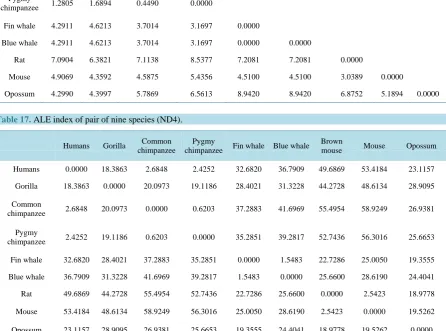
[image:8.595.65.537.207.656.2]

(9)

Table 16.

ALE index of pair of nine species (ND3).

Humans Gorilla Common

chimpanzee

Pygmy

chimpanzee Fin whale Blue whale Brown mouse Mouse Opossum

Humans 0.0000

Gorilla 0.4802 0.0000

Common

chimpanzee 1.0348 1.0749 0.0000

Pygmy

chimpanzee 1.2805 1.6894 0.4490 0.0000

Fin whale 4.2911 4.6213 3.7014 3.1697 0.0000

Blue whale 4.2911 4.6213 3.7014 3.1697 0.0000 0.0000

Rat 7.0904 6.3821 7.1138 8.5377 7.2081 7.2081 0.0000

Mouse 4.9069 4.3592 4.5875 5.4356 4.5100 4.5100 3.0389 0.0000

[image:9.595.91.538.204.535.2]

Opossum 4.2990 4.3997 5.7869 6.5613 8.9420 8.9420 6.8752 5.1894 0.0000

Table 17.

ALE index of pair of nine species (ND4).

chimpanzee

Pygmy

chimpanzee Fin whale Blue whale

Brown

mouse Mouse Opossum

Humans 0.0000 18.3863 2.6848 2.4252 32.6820 36.7909 49.6869 53.4184 23.1157

Gorilla 18.3863 0.0000 20.0973 19.1186 28.4021 31.3228 44.2728 48.6134 28.9095

Common

chimpanzee 2.6848 20.0973 0.0000 0.6203 37.2883 41.6969 55.4954 58.9249 26.9381

Pygmy

chimpanzee 2.4252 19.1186 0.6203 0.0000 35.2851 39.2817 52.7436 56.3016 25.6653

Fin whale 32.6820 28.4021 37.2883 35.2851 0.0000 1.5483 22.7286 25.0050 19.3555

Blue whale 36.7909 31.3228 41.6969 39.2817 1.5483 0.0000 25.6600 28.6190 24.4041

Rat 49.6869 44.2728 55.4954 52.7436 22.7286 25.6600 0.0000 2.5423 18.9778

Mouse 53.4184 48.6134 58.9249 56.3016 25.0050 28.6190 2.5423 0.0000 19.5262

Opossum 23.1157 28.9095 26.9381 25.6653 19.3555 24.4041 18.9778 19.5262 0.0000

8. Discussion

In this paper we introduce a novel characterization for Protein Sequence using condensed matrices that are based

on average distances for pairs of bases obtained as quotients of sequential numbers and serial numbers in

pri-mary sequences. Such matrices not only offer some insight into the nature of the protein sequence but also allow

one to make qualitative and quantitative comparisons between different sequences of proteins, whether within

the same species or between different species.

The method of construction of 20 × 20 condensed matrix of the protein sequence reveals that

• The representation of the protein sequence in 20 × 20 condensed matrix is unique.

• The condensed form of representation may help in comparing two protein sequences of unequal lengths.

• It is applicable to sequence of any finite length, however large it may be.

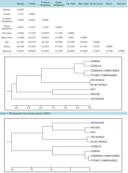
• The phylogenetic trees (Figures 1-3) of nine species of three different types of proteins (ND3, ND4 and

ND5) agree with the standard phylogenetic tree of the same species.

(10)

Table 18.

ALE index of pair of nine species (ND5).

chimpanzee

Pygmy

chimpanzee Fin whale Blue whale Brown mouse Mouse Opossum

Humans 0.0000

Gorilla 7.3253 0.0000

Common

chimpanzee 7.9996 6.8559 0.0000

Pygmy

chimpanzee 8.9492 6.5270 4.3318 0.0000

Fin whale 12.8061 15.7203 20.8209 17.1208 0.0000

Blue whale 13.3859 20.0702 20.0024 19.7006 3.4891 0.0000

Rat 64.7435 68.9178 69.1452 56.3006 50.2280 49.9102 0.0000

Mouse 60.5390 65.5209 65.3654 53.7246 43.4160 41.6367 9.6726 0.0000

[image:10.595.91.541.102.707.2]

Opossum 93.6632 90.8028 91.8434 74.5700 68.4098 70.4600 37.6871 35.1963 0.0000

Figure 1.

Phylogenetic tree of nine species (ND3).

Figure 2.

Phylogenetic tree of nine species (ND4).

HUMAN

GORILLA

COMMON CHIMPANZEE

PYGMY CHIMPANZEE

FIN WHALE

BLUE WHALE

RAT

MOUSE

OPOSSUM

0.0 0.5

1.0 1.5

2.0 2.5

3.0

OPOSSUM

MOUSE

RAT

FIN WHALE

BLUE WHALE

GORILLA

HUMAN

COMMON CHIMPANZEE

PYGMY CHIMPANZEE

0 5

10 15

(11)

[image:11.595.72.540.85.296.2]

Figure 3.

Phylogenetic tree of nine species (ND5).

9. Conclusion

Condensed matrix representation of protein sequences is a useful tool. It is applicable to comparison of protein

sequences of equal or unequal lengths and of any finite size, however large it may be. It is also an accurate one

in comparing the protein sequences of the aforesaid types.

References

[1]

Mount, D.M. (2004) Bioinformatics: Sequence and Genome Analysis. 2nd Edition, Cold Spring Harbor Laboratory

Press, Cold Spring Harbor, NY, USA.

[2]

Needleman, S.B. and Wunsch, C.D. (1970) A General Method Applicable to the Search for Similarities in the Amino

Acid Sequence of Two Proteins.

Journal of Molecular Biology

,

48 , 443-453.

http://dx.doi.org/10.1016/0022-2836(70)90057-4

[3]

Gotoh, O. (1982) An Improved Algorithm for Matching Biological Sequences.

Journal of Molecular Biology

,

162 ,

705-708.

http://dx.doi.org/10.1016/0022-2836(82)90398-9

[4]

Smith, T.F. and Waterman, M.S. (1981) Identification of Common Molecular Subsequences.

Journal of Molecular

Bi-ology,

147 , 195-197.

http://dx.doi.org/10.1016/0022-2836(81)90087-5

[5]

Bucka-Lassen, K., Caprani, O. and Hein, J. (1999) Combining Many Multiple Alignments in One Improved Alignment.

Bioinformatics

,

15 , 122-130.

http://dx.doi.org/10.1093/bioinformatics/15.2.122

[6]

Wang, L. and Jiang, T. (1994) On the Complexity of Multiple Sequence Alignment.

Journal of Computational Biology

,

1 , 337-348.

http://dx.doi.org/10.1089/cmb.1994.1.337

[7]

Shyu, C., Sheneman, L. and Foster, J.A. (2004) Multiple Sequence Alignment with Evolutionary Computation.

Genetic

Programming and Evolvable Machine

s,

5 , 121-144.

http://dx.doi.org/10.1023/B:GENP.0000023684.05565.78

[8]

Higgins, D.G. and Sharp, P.M. (1988) CLUSTAL: A Package for Performing Multiple Sequence Alignment on a

Mi-cro-Computer.

Gene

,

73 , 237-244.

http://dx.doi.org/10.1016/0378-1119(88)90330-7

[9]

Edgar, R.C. (2004) MUSCLE: Multiple Sequence Alignment with High Accuracy and High Throughput.

Nucleic Acids

Research

,

32 , 1792-1797.

http://dx.doi.org/10.1093/nar/gkh340

[10]

Katoh, K., Misawa, K., Kuma, K.-I. and Miyata, T. (2002) MAFFT: A Novel Method for Rapid Multiple Sequence

Alignment Based on Fast Fourier Transform.

Nucleic Acids Research

,

30 , 3059-3066.

http://dx.doi.org/10.1093/nar/gkf436

[11]

Notredame, C., Higgins, D.G. and Heringa, J. (2000) T-Coffee: A Novel Method for Fast and Accurate Multiple

Se-quence Alignment.

Journal of Molecular Biology

,

302 , 205-217.

http://dx.doi.org/10.1006/jmbi.2000.4042

[12]

Pham, T.D. and Zuegg, J. (2004) A Probabilistic Measure for Alignment-Free Sequence Comparison.

Bioinformatics

,

20 , 3455-3461.

http://dx.doi.org/10.1093/bioinformatics/bth426

COMMON CHIMPANZEE

PYGMY CHIMPANZEE

GORILLA

HUMAN

FIN WHALE

BLUE WHALE

MOUSE

RAT

OPOSSUM

0 5

10 15

20 25

(12)

[13]

Reinert, G., Chew, D., Sun, F. and Waterman, M.S. (2009) Alignment-Free Sequence Comparison (I): Statistics and

Power.

Journal of Computational Biology

,

16 , 1615-1634.

http://dx.doi.org/10.1089/cmb.2009.0198

[14]

Vinga, S. and Almeida, J. (2003) Alignment-Free Sequence Comparison—A Review.

Bioinformatics

,

19 , 513-523.

http://dx.doi.org/10.1093/bioinformatics/btg005

[15]

Nandy, A., Harle, M. and Basak, S.C. (2006) Mathematical Descriptors of DNA Sequences: Development and

Appli-cations. ARKIVOC, (ix) 211-238.

[16]

Luo, J., Guo, J. and Li, Y. (2010) A New Graphical Representation and Its Application in Similarity/Dissimilarity

Analysis of DNA Sequences. 4

th International Conference on Bioinformatics and Biomedical Engineering

, Chengdu,

18-20 June 2010, 1-5.

http://dx.doi.org/10.1109/icbbe.2010.5515203

[17]

Li, C., Xing, L.L. and Wang, X. (2008) 2-D Graphical Representation of Protein Sequences and Its Application to

Co-ronavirus Phylogeny.

BMB Reports

,

41 , 217-222.

http://dx.doi.org/10.5483/BMBRep.2008.41.3.217

[18]

Randić, M., Vračko, M., Novič, M. and Plavšić, D. (2009) Spectral Representation of Reduced Protein Models.

SAR

and QSAR in Environmental Research

,

20 , 415-427.

http://dx.doi.org/10.1080/10629360903278685

[19]

Randić, M., Mehulić, K., Vukičević, D., Pisanski, T., Vikić-Topić, D. and Plavšić, D. (2009) Graphical Representation

of Proteins as Four-Color Maps and Their Numerical Characterization.

Journal of Molecular Graphics and Modelling

,

27 , 637-641.

http://dx.doi.org/10.1016/j.jmgm.2008.10.004

[20]

Bai, F. and Wang, T. (2006) On Graphical and Numerical Representation of Protein Sequences.

Journal of

Biomolecu-lar Structure and Dynamics

,

23 , 537-545.

http://dx.doi.org/10.1080/07391102.2006.10507078

[21]

Randi

ć, M. (2007) 2-D Graphical Representation of Proteins Based on Physico-Chemical Properties of Amino Acids.

Chemical Physics Letters

,

440 , 291-295.

http://dx.doi.org/10.1016/j.cplett.2007.04.037

[22]

Ghosh, A. and Nandy, A. (2011) Graphical Representation and Mathematical Characterization of Protein Sequences

and Applications to Viral Proteins.

Advances in Protein Chemistry and Structural Biology

,

83 , 1-42.

http://dx.doi.org/10.1016/B978-0-12-381262-9.00001-X

[23]

Li, C., Yu, X., Yang, L., Zheng, X. and Wang, Z. (2009) 3-D Maps and Coupling Numbers for Protein Sequences.

Physica A

:

Statistical Mechanics and Its Applications

,

388 , 1967-1972.

[24]

Randi

ć, M., Zupan, J. and Vikić-Topić, D. (2007) On Representation of Proteins by Star-Like Graphs.

Journal of

Mo-lecular Graphics and Modelling

,

26 , 290-305.

[25]

Li, C., Xing, L. and Wang, X. (2008) 2-D Graphical Representation of Protein Sequences and Its Application to

Coro-navirus Phylogeny.

Journal of Biochemistry and Molecular Biology

,

41 , 217-222.

http://dx.doi.org/10.5483/bmbrep.2008.41.3.217

[26]

Wen, J. and Zhang, Y. (2009) A 2D Graphical Representation of Protein Sequence and Its Numerical Characterization.

Chemical Physics Letters

,

476 , 281-286.

http://dx.doi.org/10.1016/j.cplett.2009.06.017

[27]

Wu, Z.-C., Xiao, X. and Chou, K.-C. (2010) 2D-MH: A Web-Server for Generating Graphic Representation of Protein

Sequences Based on the Physicochemical Properties of Their Constituent Amino Acids.

Journal of Theoretical Biology

,

267 , 29-34.

http://dx.doi.org/10.1016/j.jtbi.2010.08.007

[28]

Liao, B., Sun, X. and Zeng, Q. (2010) A Novel Method for Similarity Analysis and Protein Sub-Cellular Localization

Prediction.

Bioinformatics

,

26 , 2678-2683.

http://dx.doi.org/10.1093/bioinformatics/btq521

[29]

Novi

č, M. and Randić, M. (2008) Representation of Proteins as Walks in 20-D Space.

SAR and QSAR in

Environmen-tal Research

,

19 , 317-337.

http://dx.doi.org/10.1080/10629360802085066

[30]

Qi, Z.-H., Feng, J., Qi, X.-Q. and Li, L. (2012) Application of 2D Graphic Representation of Protein Sequence Based

on Huffman Tree Method.

Computers in Biology and Medicine

,

42 , 556-563.

http://dx.doi.org/10.1016/j.compbiomed.2012.01.011

[31]

Yu, H.-J. and Huang, D.-S. (2012) Novel 20-D Descriptors of Protein Sequences and It’s Applications in Similarity

Analysis.

Chemical Physics Letters

,

531 , 261-266.

http://dx.doi.org/10.1016/j.cplett.2012.02.030

[32]

He, P.-A., Wei, J., Yao, Y. and Tie, Z. (2012) A Novel Graphical Representation of Proteins and Its Application.

Phy-sica A

:

Statistical Mechanics and Its Applications

,

391 , 93-99.

[33]

Randić, M., Novič, M. and Vračko, M. (2008) On Novel Representation of Proteins Based on Amino Acid Adjacency

Matrix.

SAR and QSAR in Environmental Research

,

19 , 339-349.

http://dx.doi.org/10.1080/10629360802085082

[34]

Randić, M., Zupan, J. and Balaban, A.T. (2004) Unique Graphical Representation of Protein Sequences Based on

Nucleotide Triplet Codons.

Chemical Physics Letters

,

397 , 247-252.

http://dx.doi.org/10.1016/j.cplett.2004.08.118

[35]

Yao, Y.-H., Kong, F., Dai, Q. and He, P.-A. (2013) A Sequence-Segmented Method Applied to the Similarity Analysis

(13)