Non parametric hidden conditional random fields for action classification

BIROn - Birkbeck Institutional Research Online

Maybank, Stephen and Raman, N. (2016) Non-parametric hidden conditional

random fields for action classification.

In: UNSPECIFIED (ed.)

2016

International Joint Conference on Neural Networks (IJCNN) - Proceedings.

New Jersey, U.S.:

IEEE Computer Society, pp.

3256-3263.

ISBN

9781509006205.

Downloaded from:

Usage Guidelines:

Please refer to usage guidelines at

or alternatively

Non-parametric Hidden Conditional Random Fields

for Action Classification

Natraj Raman, S.J.Maybank

Department of Computer Science and Information Systems, Birkbeck, University of London London, U.K.

[email protected], [email protected]

Abstract— Conditional Random Fields (CRF), a structured prediction method, combines probabilistic graphical models and discriminative classification techniques in order to predict class labels in sequence recognition problems. Its extension the Hidden Conditional Random Fields (HCRF) uses hidden state variables in order to capture intermediate structures. The number of hidden states in an HCRF must be specified a priori. This number is often not known in advance. A non-parametric extension to the HCRF, with the number of hidden states automatically inferred from data, is proposed here. This is a significant advantage over the classical HCRF since it avoids ad hoc model selection procedures. Further, the training and inference procedure is fully Bayesian eliminating the over fitting problem associated with frequentist methods. In particular, our construction is based on scale mixtures of Gaussians as priors over the HCRF parameters and makes use of Hierarchical Dirichlet Process (HDP) and Laplace distribution. The proposed inference procedure uses elliptical slice sampling, a Markov Chain Monte Carlo (MCMC) method, in order to sample optimal and sparse posterior HCRF parameters. The above technique is applied for classifying human actions that occur in depth image sequences – a challenging computer vision problem. Experiments with real world video datasets confirm the efficacy of our classification approach.

Keywords— action classification; depth video; HCRF; HDP; Laplace distribution; elliptical slice sampling;

I. INTRODUCTION

Structured prediction involves predicting a vector of output variables. It has applications in diverse areas such as sequence labelling, syntactic parsing, gene segmentation etc. The complex dependencies of the output variables are often represented using probabilistic graphical models in such applications. This includes models such as Dynamic Bayesian Networks and Markov Random Fields. For classification problems, rather than using a joint probability distribution over input and output variables, it is better to use a conditional distribution with the output variables conditioned on the inputs. This discriminative approach with the conditional distributions is preferable to the generative approach with the joint distributions, since the dependencies that involve only the input observations do not need to be modelled in the former. Conditional Random Fields (CRF) [1] combine undirected graphical modelling and discriminative classification techniques in order to represent the outputs in an accurate conditional model that is better suited for prediction tasks.

A limitation of the CRF is that it cannot capture intermediate structures. For example in a sequence labelling problem such as human action classification, an action may be composed of intermediate poses and it may be useful to incorporate the pose structure in the model. Hidden Conditional Random Fields (HCRF) [2] use intermediate hidden state variables in order to model the latent structure of the input observations. In HCRF, a joint distribution over the class label and the hidden state variables conditioned on the input observations is used. The dependencies between the hidden variables are expressed by an undirected graph as in the CRF and typically the graph is assumed to be a linear chain for tractable inference.

In the above HCRF, the number of hidden states is fixed in advance. This is a problem in general with all variants of latent variable graphical models where the number of hidden states are fixed a priori, even though this number is not known in advance. In the context of action classification, the number of intermediate poses will differ between the various actions and may depend on the number of subjects. Consequently, the exact number of hidden states is not available. The usual technique to circumvent this problem is to try different numbers of states and apply a model selection criteria such as cross validation. A better technique than this expensive ad hoc procedure is to infer the number of hidden states automatically from data.

In mixture modelling, the number of mixture components that define the input observations can be automatically inferred by using a Dirichlet Process (DP) prior. For sequences of observations, an extension to the DP, the Hierarchical Dirichlet Process (HDP) [3] can be used. In this work, the HDP prior is applied to the HCRF parameters. This results in a non-parametric HCRF model, with the number of hidden states automatically inferred based on the input observations.

mixture prior. This includes a global scale that is common to all parameters and local scales that allow deviations for each parameter. One of the local scale parameters follows an exponential distribution, resulting in a sparsity inducing Laplacian prior for the parameters. Another local scale parameter is assigned a HDP prior and ensures that only a subset of the hidden states are actually used. Elliptical slice sampling [7], a Markov Chain Monte Carlo (MCMC) technique, is used to sample the posterior parameters. This hierarchical Bayesian model, with a HDP-Laplace prior for the HCRF parameters, produces optimal and sparse posterior estimates.

Action classification, a challenging computer vision problem, has applications in diverse areas such as smart surveillance, human computer interaction and search and retrieval of videos. The 3D joint positions of a human skeleton can be estimated more robustly in depth videos [8] when compared with videos that contain RGB image sequences. These joint positions can then be used to characterize the human actions. Fig. 1 has few examples of depth images annotated with skeleton joint positions. The non-parametric HCRF technique is applied in this paper for classifying actions that occur in depth image sequences.The discriminative HCRF model, with the action class labels conditioned on the input joint positions, is well suited for action classification. A prior knowledge on the number of intermediate poses that are involved when performing an action is not necessary with the use of a non-parametric model.

Our main contribution is the definition of a fully Bayesian non-parametric HCRF model. The use of the HDP prior precludes the need to fix the number of hidden states in advance – a significant advantage. Further, the estimation of a posterior distribution rather than point estimates for the HCRF parameters eliminates over fitting. A tractable inference procedure that produces optimal and sparse posterior samples is derived. Experiments for classifying human actions are conducted on real-world datasets and results comparable to the state-of-the-art are provided.

The paper is organized as follows. Section II briefly reviews the related work, section III provides notations for HDP and HCRF, Section IV explains the non-parametric HRCF and the inference procedure. Evaluation results are in Section V and Section VI is a conclusion.

II. RELATED WORK

The various techniques used for human action recognition are reviewed in [9, 10, 11]. Many works that use depth images rely on computing sophisticated features. Relevant examples are

actionlet that represent interactions between joint positions in [25], HOJ3D that represents histogram of joint positions in [13] and the spatio-temporal representation atomic action template in [26].

The application of probabilistic graphical models for action analysis is prevalent. This includes techniques based on directed graphical models such as Hidden Markov Models (HMMs) [12, 13] and undirected graphical models such as CRF [14, 15, 23]. However, these are classical parametric models with the number of hidden states specified in advance unlike the non-parametric method used here.

There have been a few approaches based on the non-parametric HDP prior for action recognition [16, 17, 18]. These methods are based on generative techniques. The use of a discriminative approach based on CRF distinguishes our work.

The works in [19, 20] extend HCRF to be non-parametric with a DP prior. The MCMC based approach in [19] is not applicable for continuous observation features and excludes the HCRF normalization term. In contrast, our procedure handles continuous observations and takes into full account the normalization term. The variational inference based approach in [20] has non-negative constraints on the observation features. We do not enforce any such constraints on the features or parameters. Further, unlike the point estimates produced for HCRF parameters using gradient descent in [20], the work here estimates posterior distribution for the parameters.

Normal scale mixtures that induce sparsity have been used as parameter priors [6, 21]. However, these methods are applied to the classical regression problem while the work here addresses HCRF which has a more complicated model and a challenging inference task. In [5], expectation propagation is used to compute CRF parameters and average over them during inference. For tractability, the CRF partition function is approximated. In contrast, the use of a linear chain CRF lets us use the full partition function even though hidden states are incorporated into the model.

This paper brings together HCRF and non-parametric models in a fully Bayesian context for addressing the action classification problem. The novel use of a scale-mixture prior and a slice sampling procedure produces estimates of the posterior distribution for the parameters thereby reducing the chance of overfitting. To the best of our knowledge, such a Bayesian non-parametric HCRF model has not been explored in the literature before.

III. PRELIMINARIES

Background information on the DP, HDP [3, 22] is provided and the HCRF [1, 5, 23] is defined.

A. Dirichlet Processes

A Dirichlet Process, denoted by 𝐷𝑃(𝛾, 𝐻), is a useful non-parametric prior for mixture models that have no upper bound on the number of mixture components. Here 𝐻 is a base measure Fig. 1. Action classification problem. Example frames for actions horizontal

and 𝛾 ∈ ℝ+ _{is a concentration parameter that controls} variability around 𝐻. A draw 𝐺0 ~ 𝐷𝑃(𝛾, 𝐻) produces a distribution with infinitely many members. A more useful representation for a DP is through a stick breaking construction written in the following form:

𝐺0= ∑ 𝛽𝑘𝛿ℎ_𝑘 ∞

𝑘=1

(1)

𝛽𝑘 = 𝛽𝑘′∏(1 − 𝛽𝑙′) 𝑙<𝑘

𝛽𝑘′| 𝛾 ~ 𝐵𝑒𝑡𝑎(1, 𝛾) ℎ𝑘 | 𝐻 ~ 𝐻

The atoms ℎ𝑘 are drawn independently from 𝐻 and 𝛽𝑘 are the probabilities that define the mass on the atoms with

∑∞𝑘=1𝛽𝑘= 1. The probability measure 𝛽 = {𝛽𝑘}𝑘=1∞ obtained from (1) can be abbreviated as 𝛽 ~ 𝐺𝐸𝑀(𝛾).

B. Hierarchical Dirichlet Processes

HDP is the hierarchical extension to the DP. It can be used to model data that originate from multiple groups but share some characteristics across the groups. Each group has a separate DP prior but the groups are linked through a common global DP. Specifically, the set {𝐺𝑗}𝑗=1𝐽 of random distributions corresponding to 𝐽 pre-specified groups are conditionally independent given a base global distribution 𝐺0.

𝐺𝑗 | 𝛼, 𝐺0 ~ 𝐷𝑃(𝛼, 𝐺0) 𝐺0| 𝛾, 𝐻 ~ 𝐷𝑃(𝛾, 𝐻) (2)

As in (1), the HDP can be represented using a stick breaking construction as below using probability measures 𝜈𝑗= {𝜈𝑗𝑘}𝑘=1∞ .

𝐺𝑗= ∑ 𝜈𝑗𝑘𝛿ℎ_𝑘 ∞

𝑘=1

(3)

𝜈𝑗 | 𝛼, 𝛽 ~ 𝐷𝑃(𝛼, 𝛽)

𝛽 | 𝛾 ~ 𝐺𝐸𝑀(𝛾) ℎ𝑘 | 𝐻 ~ 𝐻

C. Parametric HCRF

Assume that a set of training pairs {(𝒙𝑛_{, 𝑦}𝑛_)} 𝑛=1

𝑁 _{is given.} For a particular training pair, 𝒙 = {𝑥𝑡}𝑡=1𝑇 is a list of observations and 𝑦 ∈ { 1 … 𝑐 … 𝐶} is its corresponding label. For example, in action classification, 𝒙 is the input image sequence and 𝑦 is the action class.

For any input 𝒙, let there be an associated list of hidden variables 𝒛 = {𝑧𝑡}𝑡=1𝑇 with 𝑧𝑡 ∈ { 1 … 𝑘 … 𝐾}. These hidden variables are not observed and represent one of the 𝐾 possible latent states associated with an input observation. For example, the latent state may correspond to an action pose. An HCRF models the conditional probability of a class label given the input observations as:

𝑝(𝑦 | 𝒙; 𝜽) = ∑ 𝑝(𝑦, 𝒛 | 𝒙; 𝜽)

𝒛

= ∑ exp {𝜙(𝑦, 𝒛, 𝒙; 𝜽)}𝒛 ∑ exp {𝜙(𝑦′_{, 𝒛, 𝒙; 𝜽)}}

𝑦′_,𝒛

(4)

The potential function 𝜙(𝑦, 𝒛, 𝒙; 𝜽) ∈ ℝ, parameterized by

𝜽, measures the compatibility between a label, a configuration of the hidden states and an observation vector. The denominator term in (4) is often referred as a partition function.

The structural constraints are encoded in an undirected graph. The hidden variables correspond to the graph nodes and the links between hidden variables correspond to the graph edges. Although the graph can be defined arbitrarily, in this work it is a linear chain that captures temporal dynamics. Hence the edges correspond to pairwise discrepancies between the hidden variables at time 𝑡 − 1 and 𝑡. For such an HCRF, the potential function can be defined as:

𝜙(𝑦, 𝒛, 𝒙; 𝜽) = ∑ 𝜃𝑥_{(𝑦, 𝑧}

𝑡) . 𝜑(𝒙, 𝑡) + 𝜃𝑦(𝑦, 𝑧𝑡) 𝑇

𝑡=1

+ 𝜃𝑒_{(𝑦, 𝑧}

𝑡−1, 𝑧𝑡)

(5)

The parameter vector 𝜽 is made up of three components:

𝜽 = (𝜃𝑥_{, 𝜃}𝑦_{, 𝜃}𝑒_{) and let the total number of parameters be 𝐿.} The inner product 𝜃𝑥_{(𝑐, 𝑘) . 𝜑(𝒙, 𝑡) is a measure of the} compatibility between the input observations at time 𝑡, a hidden state 𝑘 and a class label 𝑐. Each real valued parameter 𝜃𝑦_{(𝑐, 𝑘)} measures the compatibility between a label 𝑐 and a hidden state

𝑘 while 𝜃𝑒_{(𝑐, 𝑘}′_{, 𝑘) measures the compatibility between a label}

𝑐 and hidden states 𝑘′ _{and 𝑘. Here 𝜑(𝒙, 𝑡) ∈ ℝ}𝐷 _{is a vector} that can include any input feature and each 𝜃𝑥_{(𝑐, 𝑘) is a 𝐷} length vector of parameters. We can alternatively write 𝜃𝑥_(𝑘) to exclude a class label while measuring the input observations compatibility. In order to obtain a point estimate of 𝜽, typically the following regularized log likelihood function is maximized in an HCRF.

𝐿(𝜽) = ∑ log 𝑝(𝑦𝑛 _{| 𝒙}𝑛_{; 𝜽)} 𝑁

𝑛=1

− 1

2𝜎2‖𝜽‖2 (6)

IV. BAYESIAN NON-PARAMETRIC HCRF

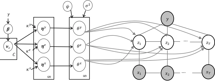
We discuss the priors that are used for the parameters and the posterior inference procedure in this section. Fig. 2 provides a graphical representation of the model.

A. Normal Scale Mixture Priors

settings, it is preferable to induce sparsity in the parameter estimates.

In the Bayesian HCRF, the posterior distribution of the parameters 𝜽 must be estimated. Instead of the 𝐿2 norm, if the likelihood function in (6) had a 𝐿1 norm penalty, then the parameters correspond to the mode of a posterior distribution obtained under a shrinkage prior [6]. Many such priors can be represented as a global-local scale mixture of Gaussians:

𝜃𝑙 ~ 𝒩(0, 𝜓𝑙𝜎2) 𝑙 = 1 … 𝐿

(7)

𝜓𝑙 ~ 𝑓 𝜎2 ~ 𝑔

Here 𝒩(𝜇, Σ) is a normal distribution with mean 𝜇 and variance

Σ. The term 𝜎2 _{is a global scale that is common to all the} parameters. The term 𝜓𝑙 is a local scale that is specific to each parameter. The prior distributions for 𝜓𝑙 and 𝜎2 are given by 𝑓 and 𝑔 respectively. The Laplacian prior has a density that is concentrated near zero with heavy tails and often produces sparse parameter estimates. Following [6, 21], if 𝑓 is the exponential distribution and 𝜓𝑙 ~ 𝐸𝑥𝑝(1/2), it implies that

𝜃𝑙 ~ 𝐷𝐸(𝜎) where 𝐷𝐸(𝑎) is a zero mean double exponential or Laplace distribution with scale 𝑎. The global scale 𝜎2 _{can be} assigned any conjugate prior such as Inverse Gamma.

In the non-parametric HRCF, the number of hidden states is unbounded and potentially 𝐾 = ∞. As discussed in III A, by using a DP prior, infinitely many members can be produced with a probability associated with each member. Since the parameters are made up of three different components, an HDP prior provides the necessary flexibility to have component specific probabilities for these members. Intuitively, there is an overall probability for being in a hidden state 𝑘, but this probability may be different for class labels 𝑐 and 𝑐′_{. Further within a same class} label 𝑐, these probabilities may be different between 𝜃𝑥 _{and 𝜃}𝑒

components. Consequently, a two level HDP prior is defined as follows:

𝜼𝑥_{(𝑐, 𝑑) | 𝝂}

𝑐 ~ 𝐷𝑃(𝜅𝑥, 𝝂𝑐) 𝑐 = 1 … 𝐶, 𝑑 = 1 … 𝐷

(8)

𝜼𝑦_{(𝑐) | 𝝂}

𝑐 ~ 𝐷𝑃(𝜅𝑦, 𝝂𝑐) 𝑐 = 1 … 𝐶

𝜼𝑒_{(𝑐, 𝑘}′_{) | 𝝂}

𝑐 ~ 𝐷𝑃(𝜅𝑒, 𝝂𝑐) 𝑐 = 1 … 𝐶, 𝑘′= 1 … ∞

𝝂𝑐 | 𝜷 ~ 𝐷𝑃(𝛼, 𝜷) 𝑐 = 1 … 𝐶

𝜷 |

𝛾

𝛾

The variable 𝜷 represents the overall probabilities of the hidden states and 𝝂𝑐 represents how these probabilities differ for each class label. The variables 𝜼𝑥_{, 𝜼}𝑦_{, 𝜼}𝑒 _{represent the state} probabilities corresponding to the different components

𝜃𝑥_{, 𝜃}𝑦_{, 𝜃}𝑒 _{. Let 𝐻𝐷𝑃(𝛾, 𝛼, 𝜅}𝑥_{, 𝜅}𝑦_{, 𝜅}𝑒_{) denote (𝜼}𝑥_{, 𝜼}𝑦_{, 𝜼}𝑒₎ obtained based on (8) using the hyper parameters 𝛾, 𝛼, 𝜅𝑥_{, 𝜅}𝑦_{, 𝜅}𝑒_. By introducing an additional local scale in (7), the HDP-Laplace prior for the HCRF parameters is specified in a hierarchical fashion as:

𝜃𝑙 ~ 𝒩(0, 𝜓𝑙𝜼𝑙𝜎2) 𝑙 = 1 … 𝐿

(9)

𝜼 ~ 𝐻𝐷𝑃(𝛾, 𝛼, 𝜅𝑥_{, 𝜅}𝑦_{, 𝜅}𝑒₎

𝜓𝑙 ~ 𝐸𝑥𝑝(1/2) 𝜎2 ~ 𝐼𝑛𝑣𝐺𝑎𝑚𝑚𝑎(𝑎, 𝑏)

B. Posterior Inference

It is intractable to compute the exact posterior and hence Gibbs sampling is used to sample the posteriors. We resort to the

𝑦

𝑧1 𝑧2 𝑧𝑇

𝑥1 𝑥2 𝑥𝑇

...

...

𝜓 𝜎2

𝜷

𝝂𝑐 𝐶 𝛾

𝜃𝑦

𝜃𝑒

𝜃𝑥

∞ 𝜼𝑦

𝜼𝑒

𝜼𝑥

∞ 𝜅𝑦

𝜅𝑥 𝜅𝑒

truncated approximation of DP for computational efficiency. Specifically we use the weak limit approximation [22] and let

𝐺𝐸𝑀(𝛾) ≜ 𝐷𝑖𝑟(𝛾 𝐾, …

𝛾 𝐾)

(10)

𝐷𝑃(𝛼, 𝜷) ≜ 𝐷𝑖𝑟(𝛼𝛽1, … 𝛼𝛽𝐾)

Here 𝐷𝑖𝑟 is the Dirichlet distribution and 𝐾 is an upper bound on the number of hidden states and is set to a large value. The prior induced by HDP leads to only a subset of states from the

𝐾 possible states being actually used. This approximation allows treating the entire model as though it is finite but as 𝐾 → ∞, the marginal distribution approaches the DP.

After initializing the variables from their respective prior distributions, our sampler cycles through as follows:

1) Sample𝒛 | 𝜽: The weak limit approximation reduces the non-parametric HCRF to a finite HCRF. Hence the hidden state sequence in (4) can be efficiently block sampled based on the standard forward backward procedure [1]. Based on 𝒛 , the count matrices

𝑁𝑥_{, 𝑁}𝑦_{, 𝑁}𝑒 _{that maintain the number of hidden states} visited for each parameter group is computed. For example, 𝑁𝑒_{∈ ℤ}𝐶×𝐾×𝐾 _{records the number of} transitions from hidden state 𝑘′ _{to 𝑘 for a class label 𝑐.} These matrices are useful for collecting posterior samples of the HDP variables.

2) Sample𝜽 | 𝜓, 𝜼, 𝜎2_{: There is no closed form solution} for sampling 𝜽 based on the likelihood function in (4). Slice sampling methods provide alternate solutions for sampling from a pdf when the pdf is known up to a scale factor. If the pdf is defined as a product of likelihood and a zero mean normal prior, then Elliptical Slice Sampling (ESS) [7] can be used to efficiently sample posteriors for even high dimensional variables. Since the prior in (9) is a zero mean normal prior, we use ESS for block sampling the posterior 𝜽 based on the conditional likelihood in (4).

3) Sample𝜓 | 𝜽, 𝜼, 𝜎2_{: The conditional posterior of 𝜓 can} be block sampled efficiently by independently sampling

𝜓𝑙 from an Inverse Gaussian distribution 𝐼𝐺(𝜼𝒍𝜎 2 |𝜃𝒍|, 1)

[6,21].

4) Sample𝜼 | 𝜽 : By using the count matrices 𝑁𝑥_{, 𝑁}𝑦_{, 𝑁}𝑒 the variables 𝜷, 𝝂, 𝜼𝑥_{, 𝜼}𝑦_{, 𝜼}𝑒 _{can be sampled using the} standard HDP posterior computation technique [3, 22]. 5) Sample 𝜎2 _{: The update here is conjugate and a}

procedure similar to [21] can be followed.

6) Sample 𝛾, 𝛼, 𝜅𝑥_{, 𝜅}𝑦_{, 𝜅}𝑒_{| 𝜷, 𝝂, 𝜼 : The concentration} hyper parameters are re-sampled conditioned on the HDP variables and the count matrices based on the standard procedure in [3].

C. Prediction

The 𝑀 posterior samples collected for 𝜽 are used for prediction. Given a new test input 𝒙′_{, and a posterior sample}

𝜽(𝒎)the class label can be predicted as:

𝑦′_{= argmax}

𝑦=1…𝐶 𝑝(𝑦 |𝒙

′_;

_𝜽

(𝒎)) ₍₁₁₎

The mode of the class labels predicted for all the posterior samples can be used as the final label. The estimation of a posterior distribution for the parameters with the Bayesian approach provides an opportunity for model averaging during prediction.

V. EXPERIMENTS

The above model is evaluated on the Kinect Activity Recognition Dataset (KARD) [12] and the Cornell Activity Dataset (CAD-60) [24]. These datasets contain depth image sequences recorded using a single Microsoft Kinect sensor. The human silhouette can be extracted robustly from a depth image and the datasets contain annotated 3D joint positions of the human skeleton. These joint positions, estimated similar to the procedure in [8], may contain errors and hence the inputs are noisy. The datasets contain actions performed by different subjects but each action involves only one subject.

Evaluations are performed both for the setting where an instance of the subject has already been seen during training and for the setting where the subject is new during testing. The former is referred as Seen while the latter as New. In the S-Seen setting, about 60% of the instances corresponding to all subjects are used for training while in the S-New setting about 60% of the subjects are used for training. The rest of the training examples are used for testing in both the S-Seen and S-New settings. The hyper parameters in the Bayesian hierarchical model are assigned vague gamma priors similar to [3]. This ensures that the initial choice of the concentration parameters is not important.

A. Features

Each frame contains 15 3D joint positions with coordinates

(𝑥, 𝑦, 𝑧) in a world coordinate frame. In order to ensure invariance to uniform translation of the body, joint positions relative to the torso are used for computing the features. Although the HCRF model allows the hidden states to depend on observations from multiple frames, we use the joint positions from one frame only and 𝑥𝑡∈ ℝ42. The feature vectors computed from the joint positions relative to the torso is projected to a lower dimensional vector space using Principal Component Analysis (PCA) and the projected vector is used as the final features. The first 𝑑 components that capture at least 90% of the total variance are used. We do not include any data from the depth channel or the RGB channel in the experiments.

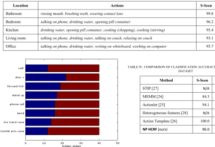
B. Posterior structure

collected. Fig. 3 shows the actual number of hidden states that were instantiated in a sampling iteration during training. Even though a large value of 40 was used for 𝐾, it can be seen that the number of hidden states that were actually used was much smaller than this number. This validates the use of DP prior. Fig. 4 shows the histogram of parameter values in a posterior sample. It can be seen that many parameter values are close to zero

indicating the sparsity of the model. During prediction, the class label is predicted for each posterior sample and the final label is selected based on the mode rather than averaging the parameter values. The block sampling procedure that is based on the forward backward algorithm has a computational cost of

𝑂(𝑇𝐾2_{) where 𝑇 is the length of the sequence and 𝐾 is the} upper bound on the number of states.

TABLE I. ACTION GROUPS IN KARD DATASET

Set A Set B Set C

horizontal arm wave high arm wave draw tick

two hand wave side kick drink

bend catch cap sit down

phone call draw tick phone call

stand up hand clap take umbrella

forward kick forward kick toss paper

draw x bend high throw

walk sit down horizontal arm wave

TABLE II. CLASSIFICATION ACCURACY (%) FOR KARD DATASET

Method Set S-Seen S-New

3D Posture [12]

Set A 95.1 93.0

Set B 89.9 90.1

Set C 84.2 81.7

NP HCRF (ours)

Set A 93.8 91.6

Set B 92.7 87.5

Set C 82.2 78.1

TABLE III. CLASSIFICATION ACCURACY (%) FOR CAD-60 DATASET

Location Actions S-Seen S-New

Bathroom rinsing mouth. brushing teeth, wearing contact lens 99.8 91.0

Bedroom talking on phone, drinking water, opening pill container 96.2 82.3

Kitchen drinking water, opening pill container, cooking (chopping), cooking (stirring) 95.4 81.9

Living room talking on phone, drinking water, talking on couch, relaxing on couch 93.1 82.5

Office talking on phone, drinking water, writing on whiteboard, working on computer 95.7 85.8

TABLE IV. COMPARISON OF CLASSIFICATION ACCURACY (%) FOR CAD-60 DATASET

Method S-Seen S-New

STIP [27] N/A 62.5

MEMM [24] 84.3 64.2

Actionlet [25] 94.1 74.7

Heterogeneous features [28] N/A 84.1

Action Template [26] 100.0 91.9

NP HCRF (ours) 96.0 84.7

C. KARD dataset

The KARD dataset contains 18 actions – horizontal arm wave, high arm wave, two hand wave, catch cap, high throw, draw x, draw tick, toss paper, forward kick, side kick, take umbrella, bend, hand clap, walk, phone call, drink, sit down and

stand up. Each action is performed by 10 different subjects and is repeated 3 times. There are 540 sequences for a total of 1 hour of videos at 30fps. The actions are grouped into three different sets of increasing complexity as in [12] for evaluation as shown in Table I.

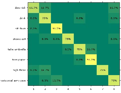
The results for KARD dataset is summarized in Table II. The confusion matrix for the three sets corresponding to the S-New setting is presented in Fig. 5, Fig. 6 and Fig. 7. The model performs better as expected for the setting where the subject has been seen. There are a few misclassifications for the S-New setting. For example, the actions horizontal arm wave and draw x involve similar motion patterns and the classifier labelled these actions incorrectly. Our results are close to the state-of-the-art in

[12] even though the latter uses a two-step procedure for training that includes sophisticated posture analysis. In contrast our method doesn’t perform any explicit posture analysis and is applicable for many other sequence labelling problems.

D. CAD-60 dataset

The CAD-60 dataset contains 12 actions –rinsing mouth,

brushing teeth, wearing contact lens, talking on phone, drinking water, opening pill container, cooking (chopping), cooking (stirring), talking on couch, relaxing on couch, writing on whiteboard and working on computer. The activities were performed by 4 different subjects and an action sequence spans about 45 seconds with an average of 1400 frames per action. The actions are grouped into five different sets based on locations

Bathroom,Bedroom, Kitchen, Living room and Office as in [24] for evaluation.

Fig. 4. Histogram plot of the parameter values in a posterior sample. The sample was collected when training the actions in bathroom location for CAD-60 dataset. The plot shows that most of the values are concentrated near zero resulting in a sparse model.

The results for CAD-60 dataset are provided in Table III and highlights that the proposed approach accurately classifies actions performed in different environments. A comparison of the results with other works in the literature is provided in Table IV. Our method outperforms [24] , [25], [27] and [28]. It is slightly less than the work in [26], but in [26] key poses are identified in advance before training. The construction of the key pose depends on the characteristics of an action. Such a method is highly data dependent and it may not be feasible to generalize this technique. In contrast, our approach is much more generic and widely applicable.

VI. CONCLUSION

Afully Bayesian non-parametric HCRF has been introduced. The number of hidden states is inferred automatically from data rather than being fixed in advance. The Bayesian structure estimates posterior distribution of the parameters and avoids over fitting. A tractable inference procedure that efficiently block samples the posteriors is provided. Experiments on action recognition datasets highlight the efficacy of using this approach. In future, we intend to apply this technique for classifying activities involving multiple subjects and objects.

REFERENCES

[1] C. Sutton, & A. McCallum, “An introduction to conditional random fields,” Machine Learning 4(4), 267-373, 2011.

[2] A. Quattoni, S. Wang, L. Morency, M. Collins, and T. Darrell, “Hidden conditional random fields,” IEEE Trans. Pattern Anal. Mach. Intell., vol. 29, no. 10, pp. 1848–1852, Oct. 2007.

[3] Y. W. Teh, M. I. Jordan, M. J. Beal, and D. M. Blei, “Hierarchical dirichlet processes,” J. Amer. Stat. Assoc., vol. 101, no. 476, pp. 1566– 1581, 2006.

[4] A. Gunawardana, M. Mahajan, A. Acero, and J. Platt, “Hidden conditional random fields for phone classification,” in Proc. Interspeech, vol. 2. 2005, pp. 1117–1120.

[5] Y. Qi, M. Szummer, and T. Minka, “Bayesian conditional random fields,” International Workshop on Artificial Intelligence and Statistics, pp. 269-276, 2005.

[6] A. Bhattacharya, D. Pati, N. S. Pillai, and D. B. Dunson. “Dirichlet-Laplace priors for optimal shrinkage,” Journal of the American Statistical Association, 2014.

[7] I. Murray, R. P. Adams, and D. J. MacKay “Elliptical slice sampling,” arXiv preprint arXiv:1001.0175, 2009.

[8] J. Shotton, A. Fitzgibbon, M. Cook, T. Sharp, M. Finocchio, R. Moore, A. Kipman, and A. Blake, “Real-time human pose recognition in parts from single depth images,” Communications of the ACM, 56(1), 116-124, 2013.

[9] J. K. Aggarwal, and M. S. Ryoo, “Human activity analysis: A review,” ACM Computing Surveys (CSUR) 43.3: 16, 2011.

[10] J. K. Aggarwal, and L. Xia, “Human activity recognition from 3d data: A review,” Pattern Recognition Letters, 48, pp. 70-80, 2014.

[11] M. Ye, Q. Zhang, L. Wang, J. Zhu, R. Yang, and J. Gall, “A survey on human motion analysis from depth data,” In Time-of-Flight and Depth Imaging. Sensors, Algorithms, and Applications, pp. 149-187, 2013. [12] S. Gaglio, G. Re, and M. Morana. “Human Activity Recognition Process

using 3-D Posture Data,” IEEE Transactions on Human-Machine Systems, 2014.

[13] L. Xia, C. Chen, and J. K. Aggarwal, “View invariant human action recognition using histograms of 3d joints,”. In Computer Vision and Pattern Recognition Workshops, pp. 20-27, 2012.

[14] Y. Wang, and G. Mori, “Max-margin hidden conditional random fields for human action recognition,” In Computer Vision and Pattern Recognition, pp. 872-879, 2009.

[15] H. Koppula and A. Saxena, "Learning spatio-temporal structure from RGB-D videos for human activity detection and anticipation," In Proceedings of the 30th International Conference on Machine Learning, pp. 792-800, 2013.

[16] A. Bargi, R. Y. Da Xu, and M. Piccardi. “An Infinite Adaptive Online Learning Model for Segmentation and Classification of Streaming Data,” Pattern Recognition, pp. 3440-3445, 2014.

[17] D. H. Hu, X. X. Zhang, J. Yin, V. W. Zheng, and Q. Yang, “Abnormal Activity Recognition Based on HDP-HMM Models,” IJCAI, pp. 1715-1720, 2009.

[18] N. Raman, and S. J. Maybank, “Action classification using a discriminative multilevel HDP-HMM,” Neurocomputing, 154, pp.149-161, 2015.

[19] K. Bousmalis, S. Zafeiriou, L. P. Morency, and M. Pantic, “Infinite hidden conditional random fields for human behavior analysis,” Neural Networks and Learning Systems, 24(1), pp.170-177, 2013.

[20] K. Bousmalis, S. Zafeiriou, L. P. Morency, M. Pantic and Z. Ghahramani, “Variational hidden conditional random fields with coupled Dirichlet process mixtures,” Machine Learning and Knowledge Discovery in Databases, pp. 531-547, 2013.

[21] T. Park and G. Casella, “The Bayesian lasso,” Journal of the American Statistical Association, 103(482), pp.681-686, 2008.

[22] E. Fox, E. Sudderth, M. Jordan, and A. Willsky. “An HDP-HMM for systems with state persistence,” Proceedings of the 25th international conference on Machine learning, ACM, pp. 312-319, 2008.

[23] S. B. Wang, A. Quattoni, L. P. Morency, D. Demirdjian, and T. Darrell, “Hidden conditional random fields for gesture recognition,” Computer Vision and Pattern Recognition, vol. 2, pp. 1521-1527, 2006.

[24] J. Sung, C. Ponce, B. Selman, and A. Saxena, “Human Activity Detection from RGBD Images,” In AAAI workshop on Pattern, Activity and Intent Recognition, 64, 2011.

[25] J. Wang, Z. Liu, Y. Wu, and J. Yuan, “Learning Actionlet Ensemble for 3D Human Action Recognition,” Pattern Analysis and Machine Intelligence, 36(5), pp. 914-927, 2014.

[26] J. Shan, and S. Akella, “3D Human Action Segmentation and Recognition using Pose Kinetic Energy,” In IEEE Workshop on Advanced Robotics and its Social Impacts, pp. 69-75, 2014.

[27] Y. Zhu, W. Chen, and G. Guo, “Evaluating spatiotemporal interest point features for depth-based action recognition,” Image and Vision Computing, 32(8), pp. 453-464, 2014.