COMMISSIONS 27 AND 42 OF THE IAU INFORMATION BULLETIN ON VARIABLE STARS

Number 6146

Konkoly Observatory Budapest

27 July 2015

HU ISSN 0374 – 0676

AO Psc TIME KEEPING

BONNARDEAU, MICHEL

MBCAA Observatory, Le Pavillon, 38930 Lalley, France, email: [email protected]

AO Piscium (RA=22h₅₅m₁₇s_{.99 DEC=}

−03◦₁₀′₄₀′′_{.0 J2000.) is an intermediate polar,} that is a subclass of cataclysmic systems in which the white dwarf is magnetized enough to module the accretion. Furthermore, the period of rotation (or spin) of the white dwarf is shorter than the orbital period and there is an accretion disc. AO Psc is one of the brightest cataclysmic, with a V mag as high as 13.2.

The orbital period isPorb = 3h.59, the rotation period of the white dwarf isProt = 805 s

and the accretion X-ray beam is reprocessed on the secondary star atmosphere, giving rise to a synodic modulation with the period Psyn such that:

1/Psyn= 1/Porb−1/Prot

i.e. Psyn = 859 s (Patterson & Price, 1981, Motch & Pakull, 1981, van Amerongen et al.,

1985 (hereafter vA85), Taylor et al., 1997).

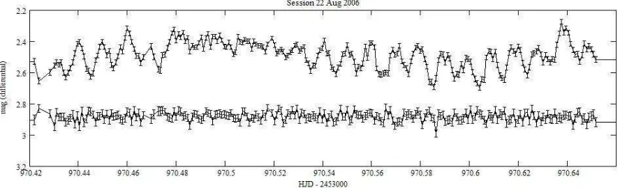
All these periodicities are visible by photometry as modulations in the light curves, the synodic modulation being usually the strongest one.

Figure 1. Upper light curve: AO Psc, Lower: the check star shifted by−0.2 mag. The error bars are the quadratic sum of the 1-sigma statistical uncertainties on the variable/check star and on the

comparison star.

ST7E camera (KAF401E CCD). The exposures were 60 s long. The images were dark substracted (using master darks of the same duration than the images and at the same temperatures) and flat corrected (MaximDL software program). For the aperture differ-ential photometry (AstroMB software package), the comparison star is GSC 5238-462. A check star, GSC 5238-347, is used to compare the standard deviations to the statistical uncertainties so as to make sure that the systematic errors are low. An example of a light curve is given Figure 1. A total of 8744 images were obtained over 74 nights.

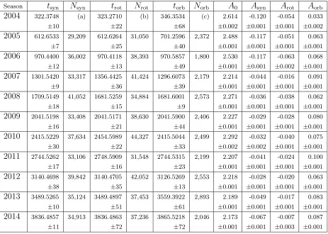
Table 1: Results of the fits and cycle counts

Season tsyn Nsyn trot Nrot torb Norb A0 Asyn Arot Aorb

2004 322.3748 (a) 323.2710 (b) 346.3534 (c) 2.614 -0.120 -0.054 0.033

±₁₀ ±₂₂ ±₆₈ ±₀

.002 ±0.001 ±0.001 ±0.002

2005 612.6533 29,209 612.6264 31,050 701.2596 2,372 2.488 -0.117 -0.051 0.063

±₇ ±₂₅ ±₄₀ ±₀

.001 ±0.001 ±0.001 ±0.001

2006 970.4400 36,002 970.4118 38,393 970.5857 1,800 2.530 -0.117 -0.063 0.068

±₁₂ ±₁₃ ±₄₉ ±₀

.001 ±0.001 ±0.002 ±0.001

2007 1301.5420 33,317 1356.4425 41,424 1296.6073 2,179 2.214 -0.044 -0.016 0.091

±₉ ±₃₆ ±₃₉ ±₀

.001 ±0.001 ±0.001 ±0.001

2008 1709.5149 41,052 1681.5259 34,884 1681.6001 2,573 2.271 -0.036 -0.038 0.062

±₁₈ ±₁₅ ±₉ ±₀

.001 ±0.001 ±0.001 ±0.001

2009 2041.5198 33,408 2041.5171 38,630 2041.5900 2,406 2.227 -0.029 -0.028 0.080

±₁₆ ±₂₁ ±₄₄ ±₀

.001 ±0.001 ±0.001 ±0.001

2010 2415.5229 37,634 2454.5989 44,327 2415.5044 2,499 2.292 -0.032 -0.040 0.075 ±₃₀ ±₂₂ ±₃₃ ±_0.002 ±_0.002 ±_0.001 ±_0.001

2011 2744.5262 33,106 2748.5909 31,548 2744.5315 2,199 2.207 -0.041 -0.024 0.100

±₁₇ ±₁₆ ±₂₃ ±₀

.001 ±0.001 ±0.001 ±0.001

2012 3140.4698 39,842 3140.4705 42,052 3126.5269 2,553 2.218 -0.028 -0.020 0.063 ±₃₈ ±₃₅ ±₁₃ ±_0.001 ±_0.001 ±_0.001 ±_0.001

2013 3489.5265 35,124 3489.4897 37,453 3559.3922 2,893 2.189 -0.049 -0.017 0.083

±₁₀ ±₅₁ ±₆₁ ±₀

.001 ±0.001 ±0.001 ±0.001

2014 3836.4857 34,913 3836.4863 37,236 3865.5218 2,046 2.173 -0.067 -0.007 0.087

±₁₁ ±₇₂ ±₇₂ ±₀

.001 ±0.001 ±0.003 ±0.001

the txxx are in HJD − 2,453,000 with the uncertainties in seconds,

the Nxxx for one season is the difference with the previous season,

the Axxx are in mag.

(a) 819,882 cycles from the 0 of vA85, 83,170 cycles from the 2002 measurement of Williams (2003) (hereafter W03).

(b) 905,581 cycles from the 0 of vA85, 711,933 cycles from the 1986 measurement of Kaluzny & Semeniuk (1988) (hereafter KS88).

(c) 56,689 cycles from the 0 of vA85 +Porb/2, 44,495 cycles from the 1986 measurement

of KS88 + Porb/2.

The magnitudes as a function of time t are fitted by the following H(t) function: H(t) = A0+Hsyn(t) +Hrot(t) +Horb(t)

where A0 is a constant, Hsyn(t) is the synodic modulation:

Hrot(t) is the rotation modulation:

Hrot(t) =Arot[cos(π(t−trot)/Prot]2

and Horb(t) is the orbital modulation:

Horb(t) =Aorb[1 + cos(2π(t−torb)/Porb)]

TheH(t) function is fitted to the observations owing to a Monte Carlo method to test the parameters relative to the timing and, for each trial, the amplitudes are determined by a least squares method. The magnitudes are weighted with the uncertainties.

Each Monte Carlo run is made of 10 millions trials. The averages and standard devi-ations for 10 runs are given in Table 1, along with the number of cycles, Nxxx.

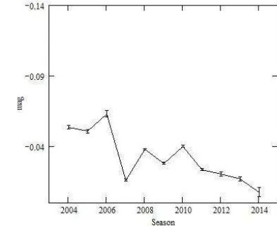
In 2007 the synodic and rotation modulations become fainter, especially the synodic one, and the orbital modulation and the non-modulated part A0 become brighter, as

shown Figures 2-5.

Figure 2. The amplitude Asyn Figure 3. The amplitudeArot

Figure 4. The amplitude A0 Figure 5. The amplitudeAorb

The times of maxima of the synodic modulation may be fitted with the function ToM(n) =Tsyn+Psynn+bsynn2. There are 26 such maxima (9 from vA85, 1 from KS88,

Fit 2. But adding the data presented here allow lifting the ambiguity: 8.9 s for the Fit 1, 15.6 s for the Fit 2. Adding the measurement of KS88 gives 9.2 s and 15.4 s respectively. Therefore, the cycle count of the Fit 1 of W03 is the right one.

The fit of the 2004-14 synodic maxima gives bsyn=−(2.544±0.043)×10−13day. This

is larger (smaller in absolute value) that the fits of W03, themselves larger than the ones of KS88 and of vA85. All the 26 maxima are then fitted with a supplementary term, γsynn3. Furthermore, they are corrected for the leap seconds due to the Earth rotation

slowing down (Eastman et al., 2010). ForTsyn in 1982 this correction is 21 s, for the first

maximum the correction is 19 s, 35 s for the last one. Tsyn is to be expressed in HJD, the

corrections are then between−2 s and +14 s. The barycentric effect of Jupiter and Saturn is neglected as it is only±4 s and cyclic (unlike the leap seconds that keep accumulating), and the other general relativistic corrections are much smaller. The least squares method gives:

bsyn =−3.020×10−13day

γsyn = 1.44×10−21day.

The fit is also done with a Monte Carlo method, so as to have a result that is in-dependent of the least squares method and to evaluate the uncertainties. For a Monte Carlo run, Tsyn, Psyn,bsyn and γsyn are chosen each in its own range; for γsyn the range is

[−10,+10]×10−21_{. 10 millions trials are computed for a run. The averages and standard}

deviations of 10 runs are:

Tsyn = 2,445,174.181,13(2) HJD

Psyn = 0.009,938,498,0(4) day

bsyn =−3.031(8)×10−13day

γsyn = 2.13(44)×10−21day.

Therefore the spinning up is slowing down. The derivative of the period is: ˙

Psyn = 2bsyn/Psyn =−6.10×10−11

and the secondary derivative of the period is: ¨

Psyn = 6γsyn/Psyn2 = 1.30×10−16day−1.

This gives the time scale: τ =Psyn/(2 ˙Psyn) = −223 kyr

and the breaking index: n=PsynP¨syn/P˙syn2 = 346.

(By comparison, for FO Aqr, one has from W03: τ = 194 kyr, n =−6431).

There are 7 orbital maxima from vA85 and one from KS88. In order to fit them with the 11 orbital minima presented here, they are corrected by adding Porb/2. A Monte

Carlo method (rather than a least squares method, so as to evaluate the uncertainties) gives the ephemeris, for the orbital minima, taking into account the leap seconds:

t(n) =Torb+Porbn

with:

Torb = 2,444,864.21809(1) HJD

Porb = 0.149,625,502,2(1) day

This is within the error bars of the ephemeris of KS88, with a better precision. An ephemeris with a quadratic term was also searched for, but with no significant improve-ment.

References:

Eastman J., Siverd R. and Gaudi B.S., 2010, PASP, 122_{, 935} Kaluzny J. and Semeniuk I., 1988,IBVS, 3145

Motch C. and Pakull M.W., 1981,A&A, 101_{, L9} Patterson J. and Price C.M., 1981, ApJ, 243_{, L83}

Taylor P., Beardmore A.P., Norton A.J., Osborne J.P. and Watson M.G., 1997,MNRAS, 289_{, 349}

van Amerongen S., Kraakman H., Damen E., Tjemkes S. and van Paradijs J., 1985,

MNRAS, 215_{, P45}

Williams G., 2003, PASP, 115_{, 618}

∗_{This version of the paper contains corrections, and differs from the one appeared on-line originally.}