Wealth effect in the US: evidence from brand new micro data

(1)

Munich Personal RePEc Archive

Wealth effect in the US: evidence from

brand new micro-data

Salotti, Simone

University of Siena

2009

Online at

https://mpra.ub.uni-muenchen.de/20966/

(2)

Wealth effect in the US: evidence from brand new micro-data

Simone Salotti

÷

This draft: February 2010

Abstract

This article investigates how wealth and capital gains affected household consumption in the

USA in the period 1989-2007. The empirical evidence brought so far by the literature is

unclear, likely because of the low quality of the data more readily available. We combine

information from the Consumer Expenditure Survey and the Survey of Consumer Finances to

perform a detailed analysis on the effects of wealth on consumption. We divide between

durables and non durables consumption, and we also investigate the roles of the different

components of household wealth, both gross and net. Our estimates indicate that there is a

significant tangible wealth effect (between one and four cents per dollar), and its economic

importance lies in the low range of the estimates of the previous empirical literature. On the

contrary, financial wealth seems to have no significant effects on consumption, apart from a

low positive effect during the Nineties (around one cent per dollar of gross wealth). The

estimation of the model with a Pooled OLS on the repeated cross sections confirms the

findings of the cross-sections estimates. Interesting features arise from the estimation of the

model dividing the sample by income quartiles, such as a decreasing wealth effect as income

rises. Overall, our results suggest that the fears of sizable reverse direct wealth effects due to

sudden declines in housing values has been overstated in previous studies.

JEL: D12, E21

Keywords: Consumption, Household Wealth, Wealth Effect

÷

(3)

1. Introduction

During the Nineties and the beginning of the new Millennium, a period of growing stock and

housing prices, the US aggregate savings rate fell considerably, leading to a renewed interest in the

understanding of its determinants. In particular, the recent literature concentrated on the effects of

household wealth on household consumption and savings, through the so called 'wealth effect'

channel. This new wave of studies aimed at understanding the possible role of wealth in

exacerbating the effects of a slowdown of the economy in case of constant or declining share and

housing prices (Paiella, 2007a). With the subprime mortgages crisis of 2007 and the following

financial and economic crisis, this scenario, from mere hypothesis, has become reality. In light of

that, the aim of our article is to explore deeply the role of household wealth on consumption and,

consequently, on savings.

Greenspan (2003) credited housing wealth, realized capital gains, and home equity borrowing with

shoring up the economy in the aftermath of the stock market collapse of 2000 and the recession of

2001, primarily through their effects on consumer spending. However, the mechanism through

which wealth directly affects consumption is not yet clearly understood: while the arguments

supporting a direct wealth effect are clear (changes in wealth directly cause changes in consumption

through their effect on households' contemporaneous budget sets), the empirical evidence brought

so far by a large literature that investigates the role of wealth shocks on consumption is unclear.

Moreover, wealth can affect consumption through the indirect channel of providing a collateral for

obtaining access to credit (Cynamon and Fazzari, 2008). Some authors claim that the decline in the

personal saving rate (that, in most developed countries, started in the middle of the Eighties) is

largely due to the significant capital gains in corporate equities experienced over this period (Juster

et al., 2005). Others conclude that there is at best a weak evidence of a stock market wealth effect,

and underline the importance of housing wealth in determining the households decisions on

consumption and savings (Case et al., 2005).

In our article we investigate the role of wealth and capital gains on household consumption in the

period 1989-2007 using a household-level dataset specifically built for this purpose, since no single

existing survey contains detailed data both on consumption and wealth. Thus, we combine

information from two different surveys: the Consumer Expenditure Survey (CES) and the Survey of

Consumer Finances (SCF). Essentially, we impute the SCF wealth variables to the CES households

(that is, we use the SCF as a donor to enrich the variables set of the CES) in order to estimate a

consumption equation with wealth, in various decompositions, as one of the main explanatory

(4)

previously for similar purposes, by Bostic et al. (2009). However, we improve the matching

methodology implemented by Bostic et al. (2009) in order to obtain a much larger dataset than

theirs, following closely the guidelines on data matching suggested by Ridder and Moffitt (2007).

As a result, we do not limit ourselves to the analysis of home owners only, and we use a richer set

of variables. Finally, our analysis includes the years 2004 and 2007, while Bostic et al. (2009) have

data up to 2001 only.

In our analysis we differentiate between financial and tangible wealth, the latter further

disaggregated into the value of the house of residence and the other real estate properties; in

addition, we investigate the role of debt on consumption decisions by studying both gross and net

wealth. Furthermore, we use information on past capital gains to investigate their direct role on

consumption, as suggested by Juster et al. (2005). This direct investigation of the effects of capital

gains on consumption has been used in early studies (Bhatia, 1972, Peek, 1983), while more recent

work has focused on wealth-based models. We have chosen to perform both, even if the results of

the capital gains specification are more prone to suffer from measurement errors, since they are

reported (in the SCF) with a lower precision with respect to the wealth stock variables. We also

investigate the consumption determinants of the older households, thanks to various interaction

terms, and we finally look at the differences between households pertaining to different income

quartiles.

The main result of our study is that tangible wealth is the main type of household wealth to

significantly and positively affect consumption. In particular, the house of residence is the part of

tangible wealth which is responsible for the highest direct wealth effect. The estimated elasticity of

consumption spending with respect to tangible wealth is between two and four cents per dollar,

which is not far from previous estimates. However, this seems to suggest that the fears of sizable

reverse direct wealth effects due to a sudden declines in housing values could have been overstated

previously (one exception being Case and Quigley, 2008), since the values involved are not

impressive. Indeed, the dynamics of the recent economic and financial crises do not reveal any

direct linkage between the declining housing prices and household consumption, rather they shed

light on the perverse mechanisms of the real estate and credit (mortgages in particular) markets.

Among the additional results, older households experience a higher wealth effect (that is, extract

more liquidity from their assets, as predicted by theory), while they have lower elasticity of

consumption with respect to income. The estimation by income quartiles shows that richer

households have a higher current income elasticity; also, their consumption paths do not take into

high consideration the value of their assets, since the estimated wealth effect for these households

(5)

The rest of this paper is organized as follows. Section 2 provides a review of the previous literature.

Section 3 describes the data used and how they were combined. Also, the econometric models are

presented. Section 4 illustrates the results. Section 5 concludes briefly.

2. The ‘wealth effect’ in the literature

There is a large literature about the wealth effect, and most of it is based on the life-cycle model

originally proposed by Ando and Modigliani (1963). According to this theory, an increase in wealth

leads the individuals to gradually increase consumption, thus lowering their savings. Also, the

propensity to consume out of wealth, whatever its form, should be the same small number (Paiella,

2007b). In practice, this is likely to be violated, “if assets are not fungible and households develop

’mental accounts’ that dictate that certain assets are more appropriate to use for current expenditure

and others for long-term saving” (Paiella, 2007b, 191). Additionally, Lettau and Ludvigson (2004)

stress that wealth shocks must be perceived as permanent in order to affect consumption. As a

result, the appraisal of the wealth effect is something that must be quantified empirically, and it has

been done in a fair number of articles that make use of either household-level or aggregate data.

Consequently, a wide range of estimates have been produced. For the U.S economy, they usually lie

between 2 and 7 cents of additional consumption per year per 1 dollar increase in household wealth.

This is consistent with the magnitude of the effect estimated by the research staff of the Board of

Governors of the Federal Reserve System, that maintains the longest and most regularly updated

wealth effect estimates for the USA.

In the latest studies, different results have been found according to the type of household wealth

analyzed, mainly dividing between house equity and financial wealth. The reason lies in the fact

that households may perceive these two kinds of wealth differently under several perspectives, and

this may influence the way it affects consumption (see Case et al., 2005, for an excellent

discussion). The empirical evidence seems to confirm this intuition, and even go beyond that. For

example, Edison and Sløk (2002) further differentiate financial wealth between technology and

non-technology segments of the stock market, finding differences in the wealth effect channel for

the USA. Case et al. (2005) study both the financial and the housing wealth effect for the US,

finding a significant effect for the latter only. Bostic et al. (2009) disaggregate household wealth

into financial, house of residence and other real estate, finding different results accordingly. Other

(6)

(2004) and Carroll et al. (2006) study the housing wealth effect, while Davis and Palumbo (2001)

concentrate on the financial wealth effect.1

The empirical appraisal of the wealth effect poses some problems, such as endogeneity and the

issue of omitted variables. Endogeneity is present in this kind of analysis, since the value of

household wealth is the result of both past savings and movements of the asset prices. In this

respect, a common weakness of the articles that investigate the wealth effect is that they use either

aggregate data or non accurate household-level data. In both cases the analysis lack proper

instruments to deal with endogeneity. In the first case there are some well known problems, such as

aggregation issues and difficulties in decomposing age, cohort and time effects, as it is well

explained by Attanasio and Banks (2001). About the second case, even if there are many sources of

household-level data for the USA, each one of them, taken singularly, has some drawbacks for the

type of analysis that is considered here. The Panel Study of Income Dynamics, (PSID, used for

example by Lehnert, 2004, Juster et al, 2005), contains data on food consumption only, and data on

household wealth have been collected since 1984 every five year only. The CES (used by Dynan

and Maki, 2001, to name one) has very detailed consumption data, but the quality of its wealth data

is low. On the other hand, the SCF does not contain detailed consumption variables, while

information on wealth is collected very accurately.

In order to overcome these well-known problems of the literature, the strategy of this paper is to

build a new household-level dataset combining CES and SCF data. We use a sample combination

procedure (explained in the next section) as a way to impute missing values of a variable which we

judge to be important in our analysis: specifically, we use it to impute the SCF wealth values to the

CES individuals for which we already have detailed consumption data. Thus, we are able to use a

very large amount of information, dealing with the problem of omitted variables and therefore

moderating the issue of endogeneity. Methods of integrating different sources of information

similar to the one that we utilized here, have been recently used by some national institutes of

statistics as a convenient way to obtain detailed datasets without having to bear the costs of

producing brand new surveys (for instance, see Rosati, 1998, D'Orazio et al., 2006, Del Boca et al.,

2005).

3. Data and model

3.1 CES and SCF data

1

(7)

In our analysis we use the wealth data from the SCF to enrich the information contained on the

CES, that already contains detailed consumption data, for the period 1989-2007.2 Then, we exploit

this “augmented” CES to perform the econometric analysis on the wealth effect, since this new

dataset is perfectly appropriate to shed light on the effects of household wealth on consumption.

The CES is collected by the Bureau of Labor Statistics (BLS) to compute the Consumer Price

Index, and contains data on up to 95 percent of total household expenditures. It is a rotating panel in

which each household is interviewed four consecutive times over a one year period. Each quarter

25% of the sample are replaced by new households. The survey contains quarterly data, thus we had

to extrapolate data on yearly consumption. Moreover, the interviews are conducted monthly about

the expenditures of the previous three months: for example, a unit interviewed in January will

appear in the same quarter of a unit interviewed in February or March, even if the reported

information will cover a slightly different period of time. This overlapping structure of the sample

complicates the operation of estimating annual consumption in many dimensions. First, the year

over which we have information for each household is different depending on the month in which

the household completes its cycle of interviews. Second, and even more important, not all

households complete the cycle of four interviews, thus they don't report all the expenditures made

in one year.

In order not to waste a vast amount of information, we have chosen to use the data of the

households present for the whole year of reference, as well as the data of the households that were

interviewed three periods or less, using the following procedure. First, we harmonized the

expenditure variables using the Consumer Price Index, differentiated for food, energy and the other

goods, in order to have all expenditures expressed with the prices of June of the reference year.

Second, we deseasonalized the quarterly measures of consumption using the ratio to moving

average method. Finally, we used a simple technique to extend these corrected quarterly

expenditures to the whole year of interest: we multiplied by four the expenditure of the households

present for one quarter only, by two the expenditure of two quarters and by four thirds the

expenditure of the households interviewed for three quarters. For the households that were present

for four quarters in a row, we just had to compute the sum across quarters. Thanks to this procedure,

we were able to obtain a dataset with more than 14,000 households for the year 2007. We checked

whether this operation led to a dataset differing from the original (quarterly) one in terms of

distributions of the variables that we used in our analysis, finding no significant difference. For each

2

(8)

household, in addition to the expenditure variables, both for durable and for non-durable goods, we

kept socio-demographic variables and annual income.3

The household wealth data that we imputed to the CES households come from the SCF, which is

triennial and is produced by the Federal Reserve Board. This survey also includes

socio-demographic information that proved valuable for the statistical matching procedure, as well as for

the estimation of the consumption models. In particular, we used data on marital status, race, age,

education and occupation of the household head, home ownership status and family size. The period

covered by the analysis starts in 1989, mainly because the SCF question frame was different in

earlier periods, and ends in 2007, with 7 periods in total. Moreover, we used the information

contained in all the five implications of the SCF (implications that derive from the multiple

imputation procedure used to approximate the distribution of missing data, as explained in

Kennickell, 1998), by performing the sample combination with the CES separately for each

implication. To correctly take into account multiple imputation, the estimation of the consumption

models were then carried out using Repeated Imputation Inference (RII), as explained by Montalto

and Sung (1996). In a few words, this method exploits all the different versions of the dataset due to

the multiple imputation technique and combines the resulting estimates in order to produce more

correct estimates in case of imputed missing values (as, in the CES case, the ones on income).

3.2 The matching procedure

The aim of the procedure is to look for similar households across the two surveys and then to attach

the wealth variables observed for the SCF households to the most similar ones in the CES, so to get

an “augmented” CES that contains detailed information on wealth in addition to the consumption

and socio-demographic variables originally collected by the BLS. In constructing and applying the

matching procedure we followed several principles and suggestions given by Ridder and Moffitt

(2007) so to make sure to produce a high quality new dataset. The details of the procedure are the

following.

We first partitioned both samples into cells based on six categorical variables in order to avoid to

match individuals that differ in important characteristics. For the year 2007, and similarly for the

other years, more than 700 cells were created using:

* Race - white, black or other;

* Marital status - married or not;

3

(9)

* Education - twelfth grade or less, high school, some college or more;

* Tenure - home owner or not;

* Occupation - not working, managers and professionals, technicians, services, operators, other;

* Family size - one, two, three or four or more people in the household.

Thanks to this highly detailed partition that took into account many different variables, we were

able to avoid the risk of matching pairs of households differing in fundamental characteristics.

Almost every cell contained individuals from both surveys, and the imputation of the wealth

variables to the CES households has been done only using SCF households pertaining to the same

cell. Thus, within every cell, we looked for the most similar individuals across the two surveys

according to the values of income and age, building a unique distance function able to measure the

differences in this two variables.4 In this way, we were able to select the pairs of households coming

from the two different surveys in which the SCF household wealth values were assigned to the CES

household. We also refined the matching by dropping the individuals for which the distance

function displayed too high value, that is, the matched individuals had non-deniable differences in

age and/or income to be paired together.5 The matching process yielded a dataset with more than

14000 observations in 2007.6

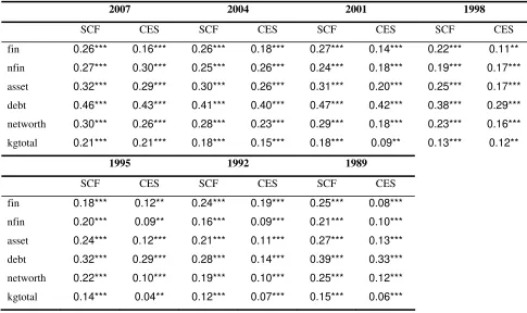
We checked the result of the matching procedure in two different ways. We verified the similarity

among the correlations between income (which is observed in both surveys) and the wealth

variables both in the SCF and in our augmented CES (after-matching). Table 1 shows that the

similarity is very high, suggesting the fact that the procedure did not change the distribution of the

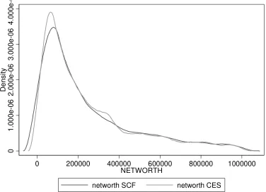
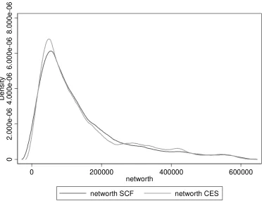
imputed variables, a signal of good quality of the overall sample combination. Furthermore, we

produced the graphs of the probability density functions of the matched variables obtained with a

kernel density estimation, finding comfortingly similar curves. Figures 1-7 report the graphs for

household net wealth: we have chosen to report this variable because it comprehends both assets

and debt, therefore it summarizes more than other variables the results of the matching procedure.

Although the two distributions do not completely overlap because not all the SCF individuals are

4

We did it performing a bivariate (income and age) propensity score matching based on Mahalanobis distance. 5

In particular, we dropped the households that fell into the top 15% of the distribution of the distance variable. We also had to build a different distance function for the groups with one or two individuals only from either one or the other survey, using the normalized logarithmic income and age, and we dropped the top 20% of households matched according to this second, and rougher, algorithm (because with few households in a cell, there was a higher probability to match pairs of households that differ significantly in their values of income and age).

6

(10)

used as donors in the matching procedure, the curves do show very similar patterns, again making

sure that the matching procedure maintained the distributional properties of the variables of interest.

We used these precautions because sample combination methods must be applied with some care,

as there are some conditions that have to be met in order not to commit errors. First, the two

different surveys must be two samples drawn from the same population (Ridder and Moffitt, 2007).

Second, there must be a set of common variables on which to condition the matching procedure, as

it is clear from the above description of the procedure. In our case, the first condition seems easy to

be met, since CES and SCF should both represent the US population. However, their sample

designs are different, since the SCF oversamples households that are likely to be wealthier, while

the CES does not. This leads to differences in the distributions of the variables of interest (in primis,

income). Consequently we had to get rid of the wealthiest households present in the SCF in order to

get comparable income distributions between the two surveys (in particular, we dropped a

percentage between 20 and 30% of the sample households with the highest income depending on

the year of reference).7 About the second condition, there are many socio-demographic variables

that are collected in both surveys, and the only problem here is to recode the variables in order to

have them measured in the same scale. This has been carried out making a large use of the

documentation that accompanies the public releases of the two surveys. The majority of these

operations of recoding were elementary. The most interesting exception has been the recoding of

the occupational sector variable for the 1989 and 1992 waves of the CES, where there is an

additional category, "self-employed", that in the SCF is not taken into account. In this case we

performed a multinomial logit estimation to impute the occupational sector to the CES individuals

labeled as "self-employed" in order to proceed with the matching with the SCF. The estimation

results were in line with the distributions of the occupational variable both in the SCF and in the

subsequent editions of the CES.

3.3 The model

Following the literature on life cycle consumption, the basic specification of our model is the

following:

'

1 2 3

log( )C =β log( )Y +β log(fin)+β log(nfin)+α Z+ε

(1)

7

(11)

where C is total consumption, Y is current income, fin is gross financial assets, and nfin is tangible

assets. Z is a vector of additional socio-demographic controls: age, educational level, a dummy for

the marital status (married or with a partner/single), two dummies for the race (one for African

Americans, the other for non-Whites) and a dummy for the occupational status (working/not

working) of the household head; the number of persons in the household; a dummy for the

homeownership status; and three different dummies for the US geographical area (Northeast,

Midwest and South, with West being the reference region). While the regional dummies are

supposed to capture macroeconomic factors, the other variables capture life cycle effects that are

likely to affect consumption. In our analysis we used a number of different specifications, in order

to investigate the role of the different components of household wealth (equation (2)), the

importance of net compared to gross wealth (equation (3)), the effects on durables and non-durables

consumption only, the effects of capital gains instead of the stocks of wealth (equation (4)). The

specifications are the following:

'

1 2 3 4

log( )C =β log( )Y +β log(fin)+β log(house)+β log(ore)+α Z+ε (2)

where tangible assets are disaggregated into house, the value of the house of residence, if owned,

and ore, the value of other real estate properties.

'

1 2 3 4

log( )C =β log( )Y +β log(netfin)+β log(house)+β log(ore)+α Z+ε (3)

where netfin is financial assets diminished by household debt.

'

1 2 3 4 5

log( )C =β log( )Y +β log(kgbus)+β log(kgstmf)+β log(kghouse)+β log(kgore)+αZ+ε (4)

where kgbus is capital gains on business activities, kgstmf on stocks and mutual funds, kghouse on

the house of residence and kgore on other real estate properties.

These four equations were also estimated with two alternative dependent variables, the logarithm of

consumption of durable and non-durable goods, the latter being more relevant and, also, more

closely related to most of the previous literature. The use of expenditure on durable goods poses

some problems, since its timing does not match the flow of services coming from the goods. The

relationship between consumption, income and wealth applies to the flow of consumption, but

(12)

flow from the existing stock” (Paiella 2007b, 198). This is why we will mainly concentrate on the

results for total and, above all, non durable goods consumption.8

The models described by the above equations were estimated cross-sectionally using data on 1989,

1992, 1995, 1998, 2001, 2004 and 2007. In the second part of the analysis we also estimated a

model by pooling data over the six surveys, adding year dummies. In all the specifications we also

added a few interaction variables in order to better grasp the wealth and consumption dynamics of

the old people. In particular, a dummy that takes the value of 1 if the household head is over 65

years old is multiplied by income and all the wealth variables. Again, the regressions were run with

the three alternative dependent variables described above.

4. Results

The results from the cross-sectional estimation of equations (1-4) are reported in Tables 2-5. For

reasons of expositional clarity, only the coefficients of the main variables of interest are reported

(complete results are available on request). We therefore reported the coefficients associated with

income and the wealth variables, including the interaction terms used to better grasp the

consumption determinants of the older households (the discussion of the latters is postponed below,

when the results of the pooled cross sections are discussed). All the estimations take into account

the multiple imputation used in the SCF using the RII (see Montalto and Sung, 1996). Very briefly,

the SCF (and consequently, our augmented CES) consists of five complete data sets because

missing data are multiply imputed. Thanks to the RII, we use information from all five data sets in

order to make valid inferences, taking into account the extra variability in the data due to

imputation.

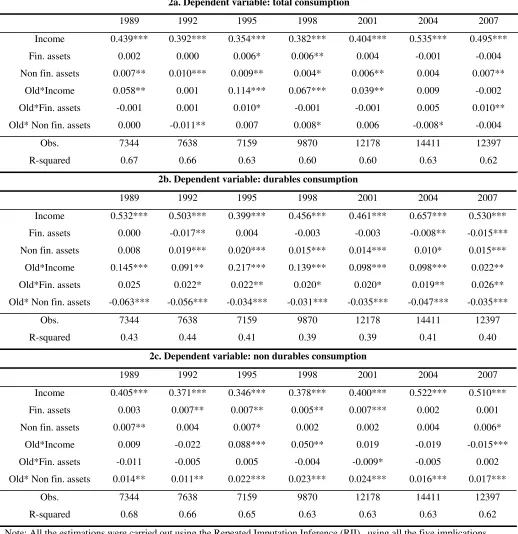
The results of the estimation of equation (1) are reported in tables 2a, 2b and 2c (as three different

dependent variables are used). Current income significantly affected consumption in the period

1989-2007, since its coefficient is always highly significant and the estimated elasticity ranges

between 0.35 and 0.53, indicating that current income plays a very important role in determining

current consumption. Turning to the household wealth coefficients, an interesting result is that the

different components do have different effects on consumption. In particular, financial wealth

positively affected consumption (both total and non-durable) during the Nineties only, while it

shows non-significant coefficients for the rest of the sample period. A possible explanation is that

8

(13)

the model captured the effects of the stock market boom that ended in 2001. However, when

significantly different from zero, the estimated elasticity of consumption to financial wealth is very

low, being it close to .01. This means that only a one cent increase in consumption is associated to a

one dollar increase in financial wealth, below most of the previous estimates that found significant

effects of this kind of wealth on consumption.

On the contrary, tangible wealth positively affects consumption throughout the whole period of

interest, even if the estimated elasticity is, again, very low (close to .01). However, we better

investigate the effects of tangible wealth in the following specifications, where we disaggregate it

into the value of the house of property and the value of the rest of real estate. We also take into

account debt considerations, when estimating equation (3). As a final consideration on the

estimation of equation (1), the surprising coefficients associated with the wealth variables in Table

2c (that is, with a negative sign) confirm the warning raised by Paiella (2007b): it is problematic to

use durable goods expenditure as the dependent variable in this kind of analysis. Therefore, we

disregard the results with this dependent variable in the rest of the discussion. However, due to the

importance of the durables part of household consumption (see Romer, 1990), throughout the whole

paper we use both total consumption and non-durables consumption as dependent variables, to

check if the results hold for the “most proper” measure of consumption (non-durables) as well as for

the most comprehensive measure (total consumption).

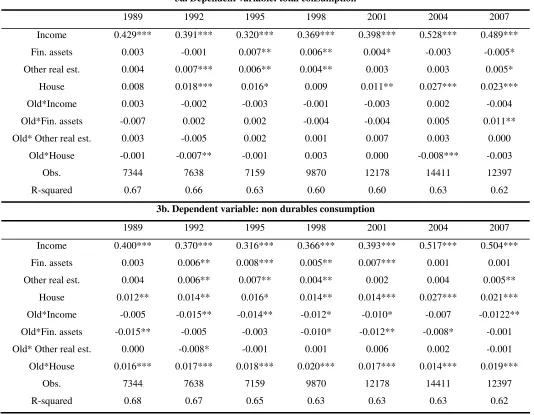
Tables 3a and 3b show the results of the estimation of equation (2), when tangible wealth is

disaggregated into the value of the house of residence and the value of other real estate. While the

results confirm the previous findings on financial wealth, they show that there are significant

differences in the way in which the value of the house of residence affects consumption, as opposed

to the rest of household’s tangible properties. The estimated elasticity for the value of the house of

residence is from three to five times larger than the one of the other real estate, reaching a wealth

effect of three cents per dollar in 2004. Moreover, while the other real estate has comparable values

across the whole sample period, the estimated elasticity for the house of residence is considerably

larger for the last two periods, 2004 and 2007. As in the case of the financial wealth coefficients of

the Nineties, this does not come as a complete surprise, because of the well known housing prices

bubble that started in 2000 and abruptly ended with the start of the recent financial crisis, in the

second half of 2007. This suggests that tangible wealth accounted for at least part of the continued

rise in consumption after the end of the financial wealth bubble in 2001, which in fact did not bring

a fall in consumption levels despite its important dimension.

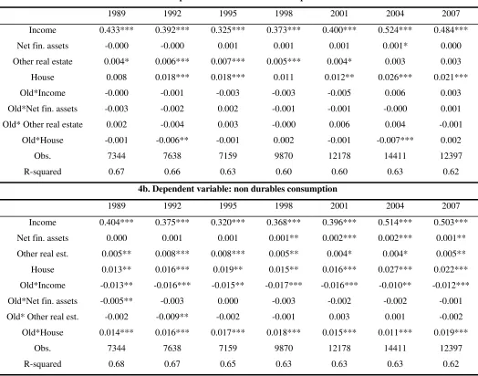
Tables 4a and 4b introduce debt considerations in the analysis, because net financial wealth is

(14)

findings for tangible wealth, while the results for the financial wealth effects are less clear-cut. The

estimated coefficients for this variable remain close to zero, but they are statistically significant in

different periods depending on the dependent variable used: there is a significant effect in the first

two periods when considering total consumption, but in the last two when considering non-durables

consumption. However, since the estimated elasticity is in all cases very low, we see this results as a

confirmation of the negligible role of financial wealth in determining consumption patterns. Also,

this suggests the possibility of some myopia on the part of households, since consumption seems

more sensitive to gross financial wealth than to net wealth.

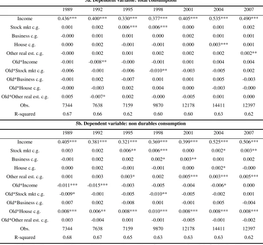
Tables 5a and 5b show the results of the estimation of equation (4), with capital gains as the wealth

variables of interest. As anticipated above, we did not expect to find important results from this

estimation, since capital gains variables are more prone than the wealth variables to severe

measurement errors that can compromise the estimation of the model. Indeed, this is confirmed by

the estimated coefficients. For all the four different types of capital gains, the associated coefficients

are always close to zero, and most of the time they are not statistically significant at standard levels.

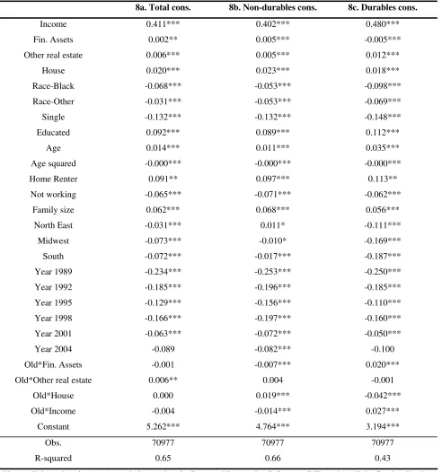
We now turn to the estimation of the pooled cross sections, shown in Tables 6 (equation (2)) and 7

(for the model described by equation (3)). The results confirm the findings of the cross-sectional

estimates, with the bigger importance of tangible wealth with respect to financial wealth, and the

higher elasticity coming from the value of the house of residence (with an estimated wealth effect

between two and three cents per dollar) with respect to the rest of the tangible assets (with an

estimated wealth effect not higher than one cent per dollar). The year dummies deserve some

considerations, keeping in mind that the reference year is 2007 (that is, the only missing dummy is

the one associated with 2007). All but one year dummies present highly significant negative

coefficients, confirming that consumption patterns are sensitive to macroeconomic conditions and

that consumption levels have risen through the sample period. The only dummy to present a

non-significant coefficient is the 2004 one, and we see this piece of evidence as a sign of the economic

crisis that hit the USA at the end of 2007, therefore causing the differences in consumption levels

between 2004 and 2007 less severe.

It is interesting to spend a few words on the results for the other explanatory variables of the model.

Most of them have significant coefficients throughout all the specifications. This is not surprising,

since a satisfactory R squared is reached in all estimations. Some results are particularly interesting

and confirm previous literature findings. For instance, the coefficients of the dummies that indicate

that the household head belongs to an ethnic minority (either Afro-American or a different one) are

always negative and economically important. A similar effect is also found for the dummy that

(15)

limiting the analysis to house-owners only, since the consumption dynamics between them and

renters are different. The results conform to the previous literature also when they show that higher

education is associated to higher consumption. The non trivial relationship between age and

consumption is confirmed by the high statistical significance of the coefficients of age and age

squared (the first positive, the second lower and negative). Finally, the regional dummies are often

associated to significant and negative coefficients, a fact that must be read bearing in mind the

region of reference (that is, whose dummy is not included) is West. Another interesting fact is the

coefficient associated to the dummy that indicates that the household head does not work, which

shows that such a condition is associated with a lower consumption, even controlling for income

and wealth. The behavior of the older households is investigated through the utilization of the

interaction terms between the “old” dummy and the income and wealth variables. The estimations

show that old people experience a higher wealth effect from the value of the house of residence

(reaching four cents per dollar of housing wealth, when non-durables consumption is the dependent

variable), while they have a lower income elasticity.

We deepen the pooled cross-sections analysis by performing an estimation dividing the sample by

income quartiles, to better understand the effects of distribution on the variables investigated. Table

8 presents the coefficients of the income and wealth variables for the estimation of equation (2),

dividing the pooled cross-sections sample by income quartiles. The results are interesting: the

consumption elasticity to income rises as we go from the lowest to the highest income quartile. At

the same time, the importance of wealth in affecting the consumption patterns decreases. This

suggests that variations of the value of the assets matter for consumption only when income is low,

while when it is high, its effects dominate the ones of wealth.

We investigated the robustness of our findings in a few ways. The results hold when we restrict our

sample to urban households only (they are almost 90% of the sample). The same is true when we

get rid of the 1% of household that are at the top and at the bottom both of the income and of the

consumption distributions. As said previously, the results are also robust to variations of the sample

combining procedure. This robustness is not surprising, since our sample is very large, and it is

unlikely that our results are driven by outliers or by small subsamples of households.

5. Conclusions

This paper analyses the strength of the wealth effect on consumption in the USA with a dataset

specifically built for this scope. We combine data from the CES and the SCF for the years

(16)

households in order to enrich the data collected in this latter survey and to perform an analysis

capable to link consumption and wealth using household-level data. This sample combination

produced a large dataset (more than 70,000 observations) capable to respect the properties of the

distributions of the variables of interest present in each of the two original survey. The resulting

dataset was then used to estimate four different specifications of a simple consumption model. The

effects of wealth were investigated using three different dependent variables: total, durables and non

durables consumption. However, the latter is the most correct measure of consumption to be used in

this kind of analysis, as widely discussed previously. Also, our dataset permits a high

disaggregation of tangible wealth, as well as a differentiation between net and gross financial

wealth. Two kinds of estimations are performed. First, the models were estimated for each

cross-section; then, a final estimation was carried out on the pooled cross-sections. In all the

specifications, a few interaction terms were used to better grasp the consumption dynamics of the

older households. The results show that tangible wealth positively affected consumption of US

households in the period 1989-2007. The estimated elasticity (between one and four cents per

dollar) lies in the low range of what constitutes the consensus on how asset market gains affect

consumer spending in the USA. It seems that households tend to consume both out of their house of

residence and out of their other real estate properties, even if the former is more important of the

latter. On the other hand, the results suggest that net financial wealth does not exert any direct effect

on household consumption, while gross financial wealth has some small effects (around one cent

per dollar), suggesting a sort of myopia on the part of households. This piece of evidence adds to

the mixed results of the previous literature, where the widest range of results has been found for this

kind of wealth. These results are confirmed both by the cross-sectional estimates and by the

estimation of the pooled cross-sections. Additional interesting results come from the estimation by

income quartiles, that shows that the consumption elasticity to income rises as we go from the

lowest to the highest income quartiles; at the same time, the importance of the wealth effect

decreases. About the older households, it seems that the wealth effect out of the house of residence

is higher for them (four cents per dollar), while their income elasticity is lower. Overall, our results

suggest that the fears of sizable reverse direct wealth effects due to a sudden decline in housing

values has been overstated in previous studies. In fact, the dynamics of the recent economic and

financial crises do not reveal any direct linkage between the declining housing prices and household

consumption, rather they shed light on the perverse mechanisms of the real estate and credit

(mortgages in particular) markets. Then, since wealth seems to play an important, though small role

in determining the consumption dynamics of the households, some other considerations must be at

(17)

countries as well, in the last twenty years. Policy makers should concentrate on these other

(18)

References

Ando, Albert , Modigliani, F., 1963. The “Life Cycle” Hypothesis of Saving: Aggregate

Implications and Tests. The American Economic Review, Vol. 53, No. 1, 55-84.

Attanasio, O., Banks, J., 2001. The Assessment: Household Saving - Issues in Theory and Policy.

Oxford Review of Economic Policy, Vol. 17, No. 1, 1-19.

Bhatia, K., 1972. Capital Gains and the Aggregate Consumption Function. American Economic

Review, 62, 866-79.

Belski, E., Prakken, J., 2004. Housing Wealth Effects: Housing’s Impact on Wealth Accumulation,

Wealth Distribution and Consumer Spending. Harvard University, Joint Center for Housing

Studies, W04-13, 2004.

Bostic, R., Gabriel, S., Painter, G., 2009. Housing Wealth, Financial Wealth, and Consumption:

New Evidence from Micro Data. Regional Science and Urban Economics, Vol. 39, 79-89.

Carroll, C., Otsuka, M., Slacalek, J., 2006. How Large is the Houseing Wealth Effect? A New

Approach. NBER Working Paper 12476.

Case, K., Quigley, J., 2008. How Housing Booms Unwind: Income Effects, Wealth Effects, and

Feedbacks through Financial Markets. Journal of Housing Policy, Vol. 8, Issue 2, 161-180.

Case, K., Quigley, J., Shiller, R., 2005. Comparing Wealth Effects: the Stock Market versus the

Housing Market. Advances in Macroeconomics, Vol. 5(1).

Cynamon, B., Fazzari, S., 2008. Household Debt in the Consumer Age: Source of Growth—Risk of

Collapse. Capitalism and Society, Vol. 3 : Iss. 2, Article 3.

Davis, M., Palumbo, M., 2001. A Primer on the Economics and Time Series Econometrics of

Wealth Effects. Board of Governors of the Federal Reserve System, Finance and Economics

(19)

D'Orazio, M., Di Zio, M., Scanu, M., 2006. Statistical Matching: Theory and Practice. Chichester,

England: Wiley.

Del Boca, D., Locatelli, M., Vuri, D., 2005. Child Care Choices of Italian Households. Review of

the Economics of the Household, No. 3, 453-477.

Dynan, K., Maki, D., 2001. Does Stock Market Wealth Matter for Consumption? Finance and

Economics Discussion Series, No. 2001.23, Washington: Board of Governors of the Federal

Reserve System.

Edison, H., Sløk, T., 2002. Stock Market Wealth Effects and the New Economy: a Cross-country

Study. International Finance 5:1, 1-22.

Greenspan, A., 2003. Remarks at the annual convention of the Independent Community Bankers of

America, Orlando, Florida,” March 4th.

Juster, T., Lupton, J., Smith, J., Stafford, F., 2005. The Decline in Household Saving and the

Wealth Effect. The Review of Economics and Statistics, 87(4), 20-27.

Kennickell, A., 1988. Multiple Imputation in the Survey of Consumer Finances.

http://www.federalreserve.gov/pubs/oss/oss2/method.html.

Lehnert, A., 2003. Housing, Consumption and Credit Constraints. Federal Reserve Board Working

Paper.

Lettau, M., Ludvigson, S., 2004. Understanding Trend and Cycle in Asset Values: Reevaluating the

Wealth Effect on Consumption. American Economic Review, 94(1), 279-299.

Montalto, C., Sung, J., 1996. Multiple Imputation in the 1992 Survey of Consumer Finances.

Financial Counseling and Planning, Vol. 7.

Paiella, M., 2007a. The Stock Market, Housing and Consumer Spending: a Survey of the Evidence

(20)

Paiella, M., 2007b. Does Wealth Affect Consumption? Evidence for Italy. Journal of

Macroeconomics, 29, pp. 189-205.

Peek, J., 1983. Capital Gains and Personal Saving Behavior. Journal of Money, Credit, and

Banking, 15, 1-23.

Rao, J., Wu, C., Yue, K., 1992. Some Recent Work on Resampling Methods for Complex Surveys.

Survey Methodology, 18(2), 209–217.

Ridder, G., Moffitt, R., 2007. The Econometrics of Data Combination. Handbook of Econometrics,

Vol. 6, 5469-5547.

Romer, C., 1990. The Great Crash and the Onset of the Great Depression. The Quarterly Journal of

Economics, Vol. 105 (3), 597-624.

Rosati, N., 1998. Matching statistico tra dati ISTAT sui consumi e dati Bankitalia sui redditi per il

(21)

[image:21.595.114.489.119.396.2]

Figures

Figure 1: Household net wealth kernel distribution, 2007

0 1. 00 0e -06 2. 00 0e -06 3. 0 0 0e -06 De ns it y

0 500000 1000000

NETWORTH

networth SCF networth CES

0 1. 00 0e -06 2. 00 0e -06 3. 00 0 e -06 4. 00 0e -06 De ns it y

0 200000 400000 600000 800000 1000000

NETWORTH

[image:21.595.112.488.474.745.2]

(22)

[image:22.595.115.488.101.368.2]

Figure 3: Household net wealth kernel distribution, 2001 0 1. 00 0e -06 2. 0 0 0e -06 3. 00 0e -06 4. 00 0e -06 De ns it y

0 200000 400000 600000 800000 1000000

networth

0 1. 00 0e -06 2. 00 0e -06 3. 00 0e -06 4 .00 0e -06 5. 00 0e -06 De ns it y

0 200000 400000 600000 800000 1000000

networth

[image:22.595.113.487.468.736.2]

(23)

[image:23.595.114.487.89.375.2]

0

2.

00

0e

-06

4.

00

0e

-0

6

6.

00

0e

-06

De

ns

it

y

0 200000 400000 600000 800000 1000000

networth

0

2.

00

0e

-0

6

4.

00

0e

-06

6.

00

0

e

-06

De

ns

it

y

0 200000 400000 600000 800000 1000000

networth

[image:23.595.113.498.466.737.2]

(24)

[image:24.595.114.486.89.374.2]

0

2.

00

0e

-06

4.

00

0e

-06

6.

00

0

e

-06

8.

00

0e

-06

De

ns

it

y

0 200000 400000 600000

networth

(25)

[image:25.595.50.535.139.427.2]

Tables

Table 1: correlations between logarithmic income and the wealth (SCF) variables

2007 2004 2001 1998

SCF CES SCF CES SCF CES SCF CES

fin 0.26*** 0.16*** 0.26*** 0.18*** 0.27*** 0.14*** 0.22*** 0.11**

nfin 0.27*** 0.30*** 0.25*** 0.26*** 0.24*** 0.18*** 0.19*** 0.17***

asset 0.32*** 0.29*** 0.30*** 0.26*** 0.31*** 0.20*** 0.25*** 0.17***

debt 0.46*** 0.43*** 0.41*** 0.40*** 0.47*** 0.42*** 0.38*** 0.29***

networth 0.30*** 0.26*** 0.28*** 0.23*** 0.29*** 0.18*** 0.23*** 0.16***

kgtotal 0.21*** 0.21*** 0.18*** 0.15*** 0.18*** 0.09** 0.13*** 0.12**

1995 1992 1989

SCF CES SCF CES SCF CES

fin 0.18*** 0.12** 0.24*** 0.19*** 0.25*** 0.08***

nfin 0.20*** 0.09** 0.16*** 0.09*** 0.21*** 0.10***

asset 0.24*** 0.12*** 0.21*** 0.11*** 0.27*** 0.13***

debt 0.32*** 0.29*** 0.28*** 0.14*** 0.39*** 0.33***

networth 0.22*** 0.10*** 0.19*** 0.10*** 0.25*** 0.12***

kgtotal 0.14*** 0.04** 0.12*** 0.07*** 0.15*** 0.06***

(26)

[image:26.595.52.570.97.631.2]

Table 2: equation (1), three different dependent variables

2a. Dependent variable: total consumption

1989 1992 1995 1998 2001 2004 2007

Income 0.439*** 0.392*** 0.354*** 0.382*** 0.404*** 0.535*** 0.495***

Fin. assets 0.002 0.000 0.006* 0.006** 0.004 -0.001 -0.004

Non fin. assets 0.007** 0.010*** 0.009** 0.004* 0.006** 0.004 0.007**

Old*Income 0.058** 0.001 0.114*** 0.067*** 0.039** 0.009 -0.002

Old*Fin. assets -0.001 0.001 0.010* -0.001 -0.001 0.005 0.010**

Old* Non fin. assets 0.000 -0.011** 0.007 0.008* 0.006 -0.008* -0.004

Obs. 7344 7638 7159 9870 12178 14411 12397

R-squared 0.67 0.66 0.63 0.60 0.60 0.63 0.62

2b. Dependent variable: durables consumption

1989 1992 1995 1998 2001 2004 2007

Income 0.532*** 0.503*** 0.399*** 0.456*** 0.461*** 0.657*** 0.530***

Fin. assets 0.000 -0.017** 0.004 -0.003 -0.003 -0.008** -0.015***

Non fin. assets 0.008 0.019*** 0.020*** 0.015*** 0.014*** 0.010* 0.015***

Old*Income 0.145*** 0.091** 0.217*** 0.139*** 0.098*** 0.098*** 0.022**

Old*Fin. assets 0.025 0.022* 0.022** 0.020* 0.020* 0.019** 0.026**

Old* Non fin. assets -0.063*** -0.056*** -0.034*** -0.031*** -0.035*** -0.047*** -0.035***

Obs. 7344 7638 7159 9870 12178 14411 12397

R-squared 0.43 0.44 0.41 0.39 0.39 0.41 0.40

2c. Dependent variable: non durables consumption

1989 1992 1995 1998 2001 2004 2007

Income 0.405*** 0.371*** 0.346*** 0.378*** 0.400*** 0.522*** 0.510***

Fin. assets 0.003 0.007** 0.007** 0.005** 0.007*** 0.002 0.001

Non fin. assets 0.007** 0.004 0.007* 0.002 0.002 0.004 0.006*

Old*Income 0.009 -0.022 0.088*** 0.050** 0.019 -0.019 -0.015***

Old*Fin. assets -0.011 -0.005 0.005 -0.004 -0.009* -0.005 0.002

Old* Non fin. assets 0.014** 0.011** 0.022*** 0.023*** 0.024*** 0.016*** 0.017***

Obs. 7344 7638 7159 9870 12178 14411 12397

R-squared 0.68 0.66 0.65 0.63 0.63 0.63 0.62

Note: All the estimations were carried out using the Repeated Imputation Inference (RII) , using all the five implications

resulting from the CES procedure of imputing missing income values. *, **, *** significant at 10, 5 and 1%

(27)

[image:27.595.50.584.101.516.2]

Table 3: equation (2), two different dependent variables

1989 1992 1995 1998 2001 2004 2007

Income 0.429*** 0.391*** 0.320*** 0.369*** 0.398*** 0.528*** 0.489***

Fin. assets 0.003 -0.001 0.007** 0.006** 0.004* -0.003 -0.005*

Other real est. 0.004 0.007*** 0.006** 0.004** 0.003 0.003 0.005*

House 0.008 0.018*** 0.016* 0.009 0.011** 0.027*** 0.023***

Old*Income 0.003 -0.002 -0.003 -0.001 -0.003 0.002 -0.004

Old*Fin. assets -0.007 0.002 0.002 -0.004 -0.004 0.005 0.011**

Old* Other real est. 0.003 -0.005 0.002 0.001 0.007 0.003 0.000

Old*House -0.001 -0.007** -0.001 0.003 0.000 -0.008*** -0.003

Obs. 7344 7638 7159 9870 12178 14411 12397

R-squared 0.67 0.66 0.63 0.60 0.60 0.63 0.62

3b. Dependent variable: non durables consumption

1989 1992 1995 1998 2001 2004 2007

Income 0.400*** 0.370*** 0.316*** 0.366*** 0.393*** 0.517*** 0.504***

Fin. assets 0.003 0.006** 0.008*** 0.005** 0.007*** 0.001 0.001

Other real est. 0.004 0.006** 0.007** 0.004** 0.002 0.004 0.005**

House 0.012** 0.014** 0.016* 0.014** 0.014*** 0.027*** 0.021***

Old*Income -0.005 -0.015** -0.014** -0.012* -0.010* -0.007 -0.0122**

Old*Fin. assets -0.015** -0.005 -0.003 -0.010* -0.012** -0.008* -0.001

Old* Other real est. 0.000 -0.008* -0.001 0.001 0.006 0.002 -0.001

Old*House 0.016*** 0.017*** 0.018*** 0.020*** 0.017*** 0.014*** 0.019***

Obs. 7344 7638 7159 9870 12178 14411 12397

R-squared 0.68 0.67 0.65 0.63 0.63 0.63 0.62

(28)

[image:28.595.55.579.103.515.2]

1989 1992 1995 1998 2001 2004 2007

Income 0.433*** 0.392*** 0.325*** 0.373*** 0.400*** 0.524*** 0.484***

Net fin. assets -0.000 -0.000 0.001 0.001 0.001 0.001* 0.000

Other real estate 0.004* 0.006*** 0.007*** 0.005*** 0.004* 0.003 0.003

House 0.008 0.018*** 0.018*** 0.011 0.012** 0.026*** 0.021***

Old*Income -0.000 -0.001 -0.003 -0.003 -0.005 0.006 0.003

Old*Net fin. assets -0.003 -0.002 0.002 -0.001 -0.001 -0.000 0.001

Old* Other real estate 0.002 -0.004 0.003 -0.000 0.006 0.004 -0.001

Old*House -0.001 -0.006** -0.001 0.002 -0.001 -0.007*** 0.002

Obs. 7344 7638 7159 9870 12178 14411 12397

R-squared 0.67 0.66 0.63 0.60 0.60 0.63 0.62

1989 1992 1995 1998 2001 2004 2007

Income 0.404*** 0.375*** 0.320*** 0.368*** 0.396*** 0.514*** 0.503***

Net fin. assets 0.000 0.001 0.001 0.001** 0.002*** 0.002*** 0.001**

Other real est. 0.005** 0.008*** 0.008*** 0.005** 0.004* 0.004* 0.005**

House 0.013** 0.016*** 0.019** 0.015** 0.016*** 0.027*** 0.022***

Old*Income -0.013** -0.016*** -0.015** -0.017*** -0.016*** -0.010** -0.012***

Old*Net fin. assets -0.005** -0.003 0.000 -0.003 -0.002 -0.002 -0.001

Old* Other real est. -0.002 -0.009** -0.002 -0.001 0.003 0.001 -0.002

Old*House 0.014*** 0.016*** 0.017*** 0.018*** 0.015*** 0.011*** 0.019***

Obs. 7344 7638 7159 9870 12178 14411 12397

R-squared 0.68 0.67 0.65 0.63 0.63 0.63 0.62

(29)

[image:29.595.56.578.99.586.2]

1989 1992 1995 1998 2001 2004 2007

Income 0.436*** 0.400*** 0.330*** 0.377*** 0.405*** 0.535*** 0.490***

Stock mkt c.g. 0.001 0.002 0.006*** 0.006*** 0.000 0.001 0.002

Business c.g. -0.000 0.001 0.001 0.000 0.002 0.001 0.001

House c.g. 0.000 0.002 -0.001 -0.001 0.000 0.003*** 0.001

Other real est. c.g. -0.000 0.002 0.001 0.002 0.002 0.002 0.002**

Old*Income -0.001 -0.008** -0.000 -0.001 0.001 0.004 0.004

Old*Stock mkt c.g. -0.006 -0.001 -0.006 -0.010** -0.003 -0.005 0.002

Old*Business c.g. -0.001 0.002 -0.007 0.001 0.001 0.005 -0.003

Old*House c.g. -0.000 -0.003 0.002 0.004 0.000 -0.003 -0.000

Old*Other real est. c.g. 0.005 -0.007* 0.002 -0.000 -0.005 0.001 0.000

Obs. 7344 7638 7159 9870 12178 14411 12397

R-squared 0.67 0.66 0.62 0.60 0.60 0.63 0.62

1989 1992 1995 1998 2001 2004 2007

Income 0.405*** 0.381*** 0.321*** 0.369*** 0.399*** 0.525*** 0.506***

Stock mkt c.g. 0.003 0.002 0.006** 0.006*** 0.000 0.002* 0.003**

Business c.g. -0.001 0.002 0.002 0.002* 0.003** 0.001 0.002

House c.g. 0.000 0.002 -0.001 -0.001 0.000 0.002* -0.000

Other real est. c.g. 0.001 0.003 0.003* 0.002 0.005*** 0.003*** 0.005***

Old*Income -0.011*** -0.015*** -0.003 -0.005 -0.004 -0.006* 0.000

Old*Stock mkt c.g. -0.009* -0.001 -0.005 -0.010** -0.005 -0.002 0.001

Old*Business c.g. 0.007 0.002 -0.008 0.001 -0.001 0.005 -0.004

Old*House c.g. 0.008*** 0.006** 0.008*** 0.010*** 0.008*** 0.008*** 0.008***

Old*Other real est. c.g. 0.003 -0.004 0.001 -0.001 -0.005 -0.001 -0.002

Obs. 7344 7638 7159 9870 12178 14411 12397

R-squared 0.68 0.67 0.65 0.63 0.63 0.63 0.62

(30)

[image:30.595.53.545.91.617.2]

Table 6: equation (2), three different dependent variables – pooled cross sections

8a. Total cons. 8b. Non-durables cons. 8c. Durables cons.

Income 0.411*** 0.402*** 0.480***

Fin. Assets 0.002** 0.005*** -0.005***

Other real estate 0.006*** 0.005*** 0.012***

House 0.020*** 0.023*** 0.018***

Race-Black -0.068*** -0.053*** -0.098***

Race-Other -0.031*** -0.053*** -0.069***

Single -0.132*** -0.132*** -0.148***

Educated 0.092*** 0.089*** 0.112***

Age 0.014*** 0.011*** 0.035***

Age squared -0.000*** -0.000*** -0.000***

Home Renter 0.091** 0.097*** 0.113**

Not working -0.065*** -0.071*** -0.062***

Family size 0.062*** 0.068*** 0.056***

North East -0.031*** 0.011* -0.111***

Midwest -0.073*** -0.010* -0.169***

South -0.072*** -0.017*** -0.187***

Year 1989 -0.234*** -0.253*** -0.250***

Year 1992 -0.185*** -0.196*** -0.185***

Year 1995 -0.129*** -0.156*** -0.110***

Year 1998 -0.166*** -0.197*** -0.160***

Year 2001 -0.063*** -0.072*** -0.050***

Year 2004 -0.089 -0.082*** -0.100

Old*Fin. Assets -0.001 -0.007*** 0.020***

Old*Other real estate 0.006** 0.004 -0.001

Old*House 0.000 0.019*** -0.042***

Old*Income -0.004 -0.014*** 0.027***

Constant 5.262*** 4.764*** 3.194***

Obs. 70977 70977 70977

R-squared 0.65 0.66 0.43

(31)

[image:31.595.52.544.91.616.2]

Table 7: equation (3), three different dependent variables – pooled cross sections

8a. Total cons. 8b. Non-durables cons. 8c. Durables cons.

Income 0.413*** 0.406*** 0.478***

Net fin. assets 0.000 0.002*** -0.003**

Other real estate 0.006*** 0.006*** 0.010***

House 0.021*** 0.025*** 0.016***

Race-Black -0.071*** -0.055*** -0.102***

Race-Other -0.033*** -0.054*** -0.070***

Single -0.133*** -0.133*** -0.148***

Educated 0.094*** 0.091*** 0.113***

Age 0.014*** 0.011*** 0.036***

Age squared -0.000*** -0.000*** -0.000***

Home Renter 0.099*** 0.103*** 0.120**

Not working -0.066*** -0.075*** -0.057***

Family size 0.061*** 0.068*** 0.056***

North East -0.031*** 0.011* -0.112***

Midwest -0.072*** -0.010* -0.169***

South -0.072*** -0.017*** -0.187***

Year 1989 -0.232*** -0.253*** -0.246***

Year 1992 -0.184*** -0.196*** -0.184***

Year 1995 -0.129*** -0.155*** -0.109

Year 1998 -0.164*** -0.195*** -0.160***

Year 2001 -0.061*** -0.071*** -0.049***

Year 2004 -0.087 -0.081 -0.098

Old*Net fin. assets -0.000 -0.004*** 0.005**

Old*Other real estate 0.006** 0.003 0.005

Old*House 0.001 0.016*** -0.034***

Old*Income -0.002 -0.016*** 0.038***

Constant 5.235*** 4.742*** 3.169***

Obs. 70977 70977 70977

R-squared 0.65 0.66 0.43

(32)

[image:32.595.59.541.92.622.2]

Table 8: equation (2), pooled OLS by income quartiles

q1 q2 q3 q4

Income 0.188*** 0.390*** 0.566*** 0.618***

Fin. assets -0.001 -0.001 -0.002 0.001

Other real est. 0.011*** 0.000 -0.001 -0.002

House 0.022** 0.014** 0.006 0.007

Old*Income 0.005 0.007 0.008 0.002

Old*Fin. assets 0.008** -0.002 0.001 0.002

Old* Other real est. -0.001 0.002 -0.005 0.011

Old*House -0.09*** -0.006* -0.008 -0.005

8b. Dependent variable: durables consumption

q1 q2 q3 q4

Income 0.332*** 0.422*** 0.590*** 0.574***

Fin. assets -0.011** -0.002 -0.005 0.001

Other real est. 0.021*** 0.000 -0.004 -0.006*

House 0.029* 0.021** 0.007 0.012

Old*Income 0.023*** 0.036*** 0.045*** 0.004

Old*Fin. assets 0.028*** 0.000 0.003 0.004

Old* Other real est. -0.009 0.004 -0.022 0.030*

Old*House -0.049*** -0.035*** -0.042*** -0.012

8c. Dependent variable: non durables consumption

q1 q2 q3 q4

Income 0.151*** 0.397*** 0.573*** 0.653***

Fin. assets 0.002 -0.001 -0.001 0.003*

Other real est. 0.009*** 0.001 0.001 -0.001

House 0.024*** 0.011** 0.006 0.003

Old*Income 0.004 -0.009 -0.10 -0.000

Old*Fin. assets 0.001 -0.006 -0.004 -0.004

Old* Other real est. -0.004 0.006 0.003 0.007

Old*House 0.004 0.016*** 0.014** 0.006