Network Averaging: a technique for determining a proxy for the dynamics of networks

Munich Personal RePEc Archive

Network Averaging: a technique for

determining a proxy for the dynamics of

networks

Bell, William Paul

University of Queensland

6 November 2009

Online at

https://mpra.ub.uni-muenchen.de/38026/

Network Averaging: a technique for determining a proxy for

the dynamics of networks

William Paul Bell

Energy Economics and Management Group

Paper presented to Complex ’09, the 9th Asia-Pacific Complex Systems Conference, Chuo

University, Tokyo, Japan, 6 November 2009.

Page 1

Network Averaging: a technique

for determining a proxy for the

dynamics of networks

William Paul Bell - University of Queensland

[email protected] - www.uq.edu..au/eemg

Abstract The main aim of this paper is to introduce the network averaging technique. This technique is introduced because accurately determining the structure of real networks can be difficult and the network averaging technique provides a proxy for real networks. A second aim is to introduce the adaptive interactive expectations (AIE) model, which uses a

‘pressure to change profit expectations index’ to replace the utility curve maximising agent concept. The AIE model has an interactive expectations network, which is difficult to determine, so suitable to illustrate network averaging. The AIE model is tested against the Dun and Bradstreet Profit Expectations Survey. The paper finds network averaging improves the predictive performance of AIE over its benchmarks: the rational expectations hypothesis and the adaptive expectations model. The network averaging technique could be adapted to other situations where there are endogenous effects acting through difficult to measure networks. The AIE model could be readily applied to other forms of expectations and as a replacement for the utility curve maximising agent. Finally, in this paper AIE models profit expectations, which are an important issue in their own right because they affect investment decisions and whether one business will extend credit to another business.

Keywords Networks, interactive, adaptive, model averaging, profit

JEL Classification B41, B52, C53, C61, C63, D81, D84, D85, E17

1 Introduction

Much of the agent based modelling simulates emergence and makes predictions against stylised facts as a form of falsification to improve their scientific veracity. However critics of agent based modelling point to the large number of parameters required for calibration. Adding to this criticism is the lack of assurance of the accurate depiction of networks. This concern is valid given that the dynamics of a network can change substantially if a link or node is incorrectly recorded. These criticisms are in part responsible for the reluctance of practitioners to adopt agent based modelling for policy development (Dawid & Fagiolo 2008, p. 352). This paper addresses these worthy criticisms by developing a network averaging technique that uses history to constrain the parameter values of models over a set of networks structures. Each network structure is a model in its own right, so

model averaging (Bates & Granger 1969) over the network structures becomes feasible to improve temporal predictive performance.

Model averaging across these network structures act as a proxy to capture the dynamics in the real network without the need to measure the network directly. Both temporal prediction, which allows benchmarking against alternative models, and constraining the parameter values using history adds to the scientific veracity of the network averaging technique. The paper uses the Adaptive Interactive Expectations (AIE) model to illustrate the technique.

2 Adaptive Interactive

Expectations Model

The AIE model combines models from the literature to produce a subjective temporal predictive expectations

model. Table

1

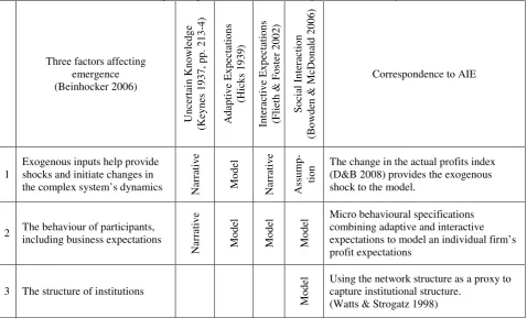
factors affecting emergence in an economic system to framework the discussion of the literature supporting the component parts of the AIE model. The three factors are: exogenous inputs, the behavior of participants and the structure of institutions. Keynes’

(1937, pp. 213-4) “uncertain knowledge” forms the

conceptual link between exogenous inputs and the behaviour of participants for the AIE model, but this conceptual link is in narrative form only. However, Hicks’ (1939) Adaptive Expectations does provide a temporal predictive model linking the two factor, which encapsulates Tversky and Kahneman’s (1974)

“adjustment and anchoring heuristic”. The AIE model uses the Adaptive Expectations model (Hicks 1939) to link the first two factors in Table

1

In comparison to the temporal predictive Adaptive Expectations model, both the Interactive Expectations (Flieth & Foster 2002) and Social Interaction (Bowden & McDonald 2006) models use stylised facts for

falsification and link the first two factors in Table

1

world network approach of Watts and Strogatz (1998). The AIE model adopts this approach also but AIE

provides for temporal prediction.

Table 1 Factors affecting emergence in an economic system and correspondence to AIE

Three factors affecting emergence (Beinhocker 2006) U nc er ta in K now le dge (K eyne s 193 7, p p. 2 13 -4) A da pt ive E xpe ct at io ns (H ic ks 1939 ) In ter act iv e E x p ect at io n s (F li et h & F os te r 2002 ) S o cia l I n te ra ctio n (B ow de n & M cD ona ld 20 06)

Correspondence to AIE

1

Exogenous inputs help provide shocks and initiate changes in

the complex system’s dynamics _Nar

ra tiv e M o d el N ar ra tiv e A ss u m p -tio

n The change in the actual profits index

(D&B 2008) provides the exogenous shock to the model.

2 The behaviour of participants,

including business expectations

N ar ra tiv e M o d el M o d el M o d

el Micro behavioural specifications _{combining adaptive and interactive}

expectations to model an individual firm’s profit expectations

3 The structure of institutions

M

o

d

el Using the network structure as a proxy to

capture institutional structure. (Watts & Strogatz 1998)

Figure 1 shows the D&B (2008) profit expectations and actual profit indices. The dataset the AIE model is tested against. The respondents to the D&B (2008) survey state whether their actual profits increased, decreased or underwent no-change the previous quarter and whether they expect their profits to increase, decrease or undergo no-change in the following quarter. The change in profit rather than level or state of profit encapsulates Kahneman and Traversky’s

(1979) prospect theory and the “primacy of change

over state” (Kahneman 2002). An approach AIE takes but at odd with utility curve maximizing agents. The Sonnenschein–Mantel–Debreu Theorem (Debreu 1959) proves the neoclassic framework is logically inconsistent, which uses the utility curve maximizing agents as a basic axiom (Arnsperger & Varoufakis 2006; Farmer & Geanakoplos 2008; Keen 2001). Farmer and Geanakoplos (2008) call for alternative approaches to the utility curve maximizing agents to

model choice. This paper introduce the ‘pressure to

change profit expectations index’ px as an alternative. To test the AIE model, the D&B (2008) profit indices are decomposed into the percentage of business with a decrease, increase and no-change in profits for both their expectations and actualization indices. Lacking a better alternative, the percentage of business expecting no-change in profits from the ABS (2002 Cat. No. 5250.0 tbl. 2) aids in the decomposition. The number

of firms or business in AIE is n = 200 because Bowden

and MacDonald (2006) use n = 200 and n = 400 in

their Social Expectations model and find little difference in the results but a large saving in computing

time. From the percentage breakdowns each business i

at time t is assigned a level of expectations ei,t of 1, 0 or

–1 to represent whether they expect profits to increase,

undergo no–change or to decrease. The actualisations

ai,t are assigned similarly. So far these assignments

reflect the D&B (2008) indices.

2.1 Justification for the pressure to

change profit expectations index p

This section makes two arguments to justify the use of the index px, rather than use probabilities.

2.1.1 The need for an Alternative Measure of Belief to Outcome or Probability

There are three aspects to why there is a need for an alternative measure of belief to outcome or probability. First, how people have an asymmetry in their attitude

toward “risk”, which is at odds with probability theory

and requires modelling with weights. Second, how

people are “ambiguity” adverse, which is at odds with

Page 3

Kahneman and Tversky (1979) introduce prospect theory as an alternative decision making theory to Von Neumann and Morgenstern’s (1944) rational choice. Kahneman and Tversky (1979) find that replacing probabilities with weights provides a more accurate description and prediction of people’s decision making,

finding people are “risk” adverse in gains but “risk”

seeking in losses.

Ellsberg (1961) provides evidence that peoples beliefs cause people to act at odds with the Bayesian approach, calling into question the applicability of conventional probabilities to beliefs. Camerer and Weber (1992) discuss ambiguity or the uncertainty about

probabilities, finding people are “ambiguity averse”.

They observe this in a dozen or so experiments confirming Ellsberg’s (1961) findings. Eichberger, Kelsey and Schipper (2009) discuss ambiguity in social

interaction, stating that ‘A decision-maker is said to

have an ambiguous belief if it is not precise enough to be represented by a single probability distribution.’ Eichberger, Kelsey and Schipper (2009) cite Knight (1921) contrasting risk where probabilities are known with ambiguity where probability can not be assigned. They claim ambiguity is common place; for example the probability of the success of a peace negotiation or

the likely impact of a new technology. However they note that Savage’s (1954) subjective decision making theory has made the distinction between ambiguity and risk from an analytical point of view obsolete because beliefs are represented by a probability distribution. This view on the demise of the distinction is consistent with Vercelli (2007, p. 21) discussed in section 2.1.2. Eichberger, Kelsey and Schipper (2009) use a Choquet (1954) expected utility framework to generalise the

subjective expected utility because “it maintains the

separation of beliefs and outcome evaluation, which makes the theory easier to apply in economics and social sciences.”

Further to the need to separate belief from probability and outcome, Figure 1 shows a persistent optimism bias as the profit expectations exceed the actual profits for almost the entire history of the D&B survey. This contrasts to Bowden and MacDonald (2006) who use a Bayesian approach to model the price movements of shares. In their model, they assume that agents find the true state of the world after a price change given a lag. Figure 1 shows that the firms never seem to learn the true state of the world. This is a form of optimism bias

and is reflected in the calculation of px, see section

2.2.1.1.

Figure 1 All–firms Profit Expectations and Actual Profits Indices

(Source: D&B 2008)

1988 1990 1992 1994 1996 1998 2000 2002 2004 2006 2008 -30

-20 -10 0 10 20 30 40 50 60 70

Quarters

P

er

c

ent

age P

rof

it

E

x

pec

tat

ion and A

c

tual

is

at

ion I

ndi

c

2.1.2 Probability in Stationary Decision Theory versus Unknowables in Adaptive Processes

The second argument for using an index rather than probabilities hinges on the more pure form of uncertainty, the unknowable. Vercelli (2007, p. 21) and Keynes (1937) make the unknowable argument using different approaches: axiomatically and the inability to measure the value of current additions to investments respectively. Vercelli (2007, p. 21) notes that the objective and subjective decision making theories may appear very different. However their implications are almost identical axiomatically and ontologically because both theories refer to a world that is familiar to the decision maker. As Lucas (1986,

p. S411) notes “the economic theory of choice is ... a

description of a ... stationary ‘point’ ... [in a] dynamic adaptive process.” At such a point, the optimal adaptation has already happened and the decision maker knows the complete list of its possible states and options, and knows the consequences of each choice for each possible state. However in an environment where there are innovations and true learning, providing novel states and outcomes that were formerly unknown, it is not possible to attribute probabilities. Such a situation requires a dynamic adaptive approach.

Keynes (1937, pp. 213-4) discusses “uncertain”

knowledge claiming that probabilities relating to the relatively distant future are not measurable because "the prospect of a European war" or "the rate of interest twenty years hence" are so uncertain that "there is no scientific basis on which to form any calculable probability whatever. We simply do not know". The probabilities of events affecting the value of current additions to capital are not measurable. Therefore, the present value of current investment cannot be calculated. He suggests that people adopt the following three strategies in the face of uncertainty.

1. Assume the present is a much more servable guide

to the future than the past and largely ignore the unknowns in the future. This is a form of exponential discounting and is reflected in the calculation of px, see section 2.2.1.3.

2.

the prices and the characteristic of existing output is a correct summing up of future prospects, unless something new and relevant comes into the picture. This is a dynamic adaptive expectations

approach and is reflected in the calculation of px,

see section 2.2.1.3.

3. Knowing our own judgement worthless, fall back

on the judgement of the rest of the world, so doing conform to the behaviour of the majority or

average, leading to a “conventional” judgement.

This is an interactive expectations approach and is

reflected in the calculation of px, see section

2.2.1.2.

2.2 Pressure to change profit

expectations index p

The px index provides a non-probabilistic method to

enable the summing of pressures that can change the profit expectations of an individual firm from three sources: interactive pressure, adaptive pressure and biases, which can be optimism, pessimism or

ambivalence. The px index is used to determine

stochastically whether a firm changes its profit expectations.

The structure of the section follows. Section 2.2.1

discusses the calculation of px. Section 2.2.2 discusses

how px is used stochastically to determine whether a

firm changes expectations. Section 2.2.3 discusses

how the maximum and minimum px is restricted to be

100 and –100 respectively.

2.2.1 Calculating the Pressure to Change Profit Expectations Index

This section discusses how the pxi,t is calculated for

each firm i each quarter t. Equation (1) shows the

calculation of the px for: (a) firms who currently expect

profits to decrease; (b) firms who currently expect no change in profits; and (c) firms who currently expect

profits to increase. The px in each equation has three

main components: the interactive and adaptive influences and the biases. The biases include optimism, pessimism and ambivalence. The interactive influence uses the difference between profit expectations of the firm and those firms linked to it; plus this difference is normalised and put to a power

ranging between 1 and 3 by increments of 0.2. The

adaptive influence uses the error between the expected profits and actual profits for the current and the previous period. This section discusses these components and compares them to the interactive expectations and adaptive expectations from which the AIE model is developed.

The structure of the section follows. Section one discusses the three biases: optimism, ambivalence and pessimism. Section two discusses the interactive influence and interactive power. Section three discusses the adaptive influences.

2.2.1.1 Biases: Optimism, Ambivalence or Pessimism

The basic tendencies β in equation (1) are, as the name

suggests, the tendency for a firm to feel pressure to change to another level of expectations. The basic

tendency to increase β+, to decrease β– and to be

neutral β0 could be interpreted respectively as

Page 5

increase is greater than the basic tendency to decrease. The AIE model does find this to be the case.

Equation (1) – Pressure to change profit expectations index (a) For firm i who currently expects profits to decrease (ei,t = –1)

The pressure to increase expectations

pxi,t= β +_{+ β}0

+ A [ ai,t – ei,t ] + A–1 [ ai,t–1 – ei,t–1 ] + I [ (Li,t +

+ Li,t

0_{) / L ]^δ}

(b) For firm i who currently expects no change in profits (ei,t = 0)

positive pressure to increase expectations and negative pressure to decrease expectations

pxi,t= β +

– β– + A [ ai,t – ei,t ] + A–1 [ ai,t–1 – ei,t–1 ] + I [( Li,t

+_{/ L )^δ}

– ( Li,t

–_{/ L )^δ]}

(c) For firm i who currently expects profits to increase (ei,t = 1)

The pressure to decrease expectations

pxi,t= β–+ β0 + A [ ei,t – ai,t ] + A–1 [ ei,t–1 – ai,t–1 ] + I [ (Li,t– + Li,t0) / L ]^δ

Where

pxi,t = pressure to change profit expectations index for firm i at time t

pxi,t ∈ [–100, 100 ]

β+

= basic tendency to increase expectations – optimism bias

β0

= basic tendency to neutral expectations – ambivalence bias

β–

= basic tendency to decrease expectations – pessimism bias A = adaptive influence this quarter

A–1 = adaptive influence last quarter

ai,t = profit actualisation of firm i at time t

where a decrease, no change or increase is –1, 0 or 1 respectively ei,t = profit expectations of firm i at time t

where a decrease, no change or increase is –1, 0 or 1 respectively I = interactive influence

L = total number of links to a node or firm (2, 4, 6, …, 22)

L+ = the number of linked firms who expect profits to increase (e = 1)

L0 = the number of linked firms who expect no change in profits (e = 0)

L– = the number of linked firms who expect profits to decrease (e = –1)

δ = interactive power (1.0, 1.2, 1.4, …, 3.0)

2.2.1.2 Interactive Influence and Interactive Power

The interactive influence I in equation (1) indicates the

influence of other firms holding differing levels of profit expectations have on the firm. Each firm is linked to other firms via a network. The total number of links to a firm L= Li,t+ + Li,t0 + Li,t– is the sum of

the links to firms that hold optimistic, ambivalent and pessimistic expectations respectively. Section 2.3

discusses the 121 network topologies (L and ρ) and

parameters ranges that AIE uses. The AIE model borrows the network naming conventions and topology parameters from Watts and Strogatz’s (1998) small world networks, the code from Wilensky (2005), and parameter increments from Bowden and McDonald (2006). This ensures that the design of the AIE model’s network builds upon the existing literature.

The interactive power δ in equation (1) varies from 1 to

3 by increments of 0.2. These increments are chosen to

test Flieth and Foster’s (2002) assumption that δ = 2.

The interactive components are adapted from Flieth and Foster (2002) and Bowden and McDonald (2006).

2.2.1.3 Adaptive Influence

The adaptive influences A and A–1 in equation (1a)

indicate the influence that the firm’s own expectations are met. The adaptive influences weights are the parameters (ai,t – ei,t) and (ai,t–1 – ei,t–1), which form a

link between the actual profits and profit expectations. For example, if the firm’s expectations are met that is

(ai,t = ei,t) and (ai,t–1 = ei,t–1), the firm has zero pressure

If the firm’s expectations are exceeded that is (ai,t > ei,t)

or (ai,t–1 > ei,t–1), the adaptive influence increases

pressure on the firm to increase its expectations. The AIE model uses the current and last quarter only, reflecting the fact that a firm lacks full information about the actual profits for the current quarter until the following quarter, so a firm behaving adaptively would use the full information available from last quarter and the partial information available about this quarter.

The adaptive expectations influence A is adapted from

Hicks’ (1939) adaptive expectations. This influence allows a connection between actual profits and profit expectations, which Flieth and Foster’s (2002) Interactive Expectations lacks.

2.2.2 Stochastically Determining the Pressure Level at which to Change Expectations

Equation (2) shows how the px in conjunction with a

random number generator and the ‘pressure levels at

which to change expectations’ p+, p++, p– and p– –

determines the level of expectations a firm holds for

the next quarter ei,t+1. These values are aged and the

process is repeated for each quarter to form a single run. The random function in equation (2) reports a random integer greater than or equal to 0, but strictly less than the pressure to change level (Wilensky 1999). The random function uses a flat distribution.

Once the AIE model calculates the expectations of each

firm for each period, the ‘profit expectations index’ of

the AIE model is calculated. Table

1

model variance between the ‘profit expectations index’

of the AIE and D&B survey for the best single run and the model averaging discussed next.

Equation (2) – Determining the pressure level at which to change expectations

(a) For firms who currently expect profits to decrease, determining the pressure level to increase expectations

if random ( p+ ) < pxi,t then ei,t+1 = 0

the firm increases expectations one level

if random ( p++ – p+ ) < ( pxi,t – p +

) then ei,t+1 = 1

the firm increases expectations two levels

(b) For firms who currently expect no change in profits determining the pressure level to increase or decrease profit expectations

if pxi,t > 0 and if random( p+ ) < abs( pxi,t ) then ei,t+1 = 1

the firm increases expectations one level

if pxi,t < 0 and if random( p– ) < abs( pxi,t ) then ei,t+1 = –1

the firm decreases expectations one level

(c) For firms who currently expect profits to increase The pressure to decrease expectations if random ( p– ) < pxi,t then ei,t+1 = 0

the firm decreases expectations one level if random ( p– – – p– ) < ( pxi,t – p– ) then ei,t+1 = –1

the firm decreases expectations two levels Where

p+ = the pressure level at which a firm increases profit expectations by 1 level

p++ = the pressure level at which a firm increases profit expectations by 2 levels

p– = the pressure level at which a firm decreases profit expectations by 1 level

p– – = the pressure level at which a firm decreases profit expectations by 2 levels

ei,t+1 = profit expectations the firm holds next quarter

2.2.3 Constraining px to ±100

Equation (3) ensures that the px does not exceed 100.

Line 1 in equation (3) shows how the px is constrained

to a maximum of 100 by setting px in equation (1a) to

100. The parameters ai,t, ei,t, ai,t–1and ei,t–1 can all take

the values 1, 0 or –1, so the maximum values for [ ai,t –

Page 7

doubling the weight of A or A–1 on the p x

, so the factor

of 2 introduced in line 2 of equation (3). The

maximum value for (Li,t+ + Li,t0) / L is 1, so a factor of

1 is introduced in line 2 of equation (3) for I. The

constraint in line 2 allows β0 to be determined in line 3

with the condition that β0 is not less than zero. This

constraint allows the elimination of β0 from the

parameter sweeping.

Equation (3) – Fixing the maximum px to 100

1. 100 >= β++ β0 + A [ ai,t – ei,t ] + A–1 [ ai,t–1 – ei,t–1 ]

+ I [ (Li,t+ + Li,t0) / L ]^δ

2. 100 >= β++ β0 + I + 2 * [ A + A–1 ]

3. β0 = 100 – ( β+ + I + 2 * [ A + A–1 ] )

Where β0

>= 0

2.3 Network Averaging

The solution space for the model variance is nonlinear and unsuitable for a simple gradient search. So, a combination of three search techniques is used: grid-gradient, threshold accepting and unconstrained nonlinear optimization. There is uncertainty over the interactive expectations network structure, so AIE

model averages over 121 network structures. The

terminology for the networks is consistent with Watts

and Strogatz (1998). The increments for the 121

networks are consistent with Bowden and MacDonald (2006): L ranges from 2 to 22 by increments of 2 and ρ

ranges from 0 to 1 by increments of 0.1. The model

variance for each of the network structures is minimized. Table 2 shows the equal weighted model averaging of the 121 network structures.

2.4 The Adaptive Expectations Model

as a Benchmark for AIE

The adaptive expectations model forms a benchmark for AIE. The adaptive expectations model is the AIE

with the interactive component set to zero that is I = 0.

The number of links is set to one L = 1 to prevent a

divide by zero error. For the aggregated adaptive expectations model a slightly lower model variance for the model averaging was found by setting the network topology to values other than L = 1 and ρ = 0. Since I

= 0, these alternate network topology settings only

indirectly affect the model variance calculation because the random functions in the model are affected by using different values. Bell (2009) discusses this issue further.

2.5 The Rational Expectations

Hypothesis as a Benchmark for AIE

The REH provides a benchmark for AIE and needs to be made operational. Sargent (2008, p. 1) asserts in rational expectations that outcomes do not differ systematically (i.e., regularly or predictable) from what

people expect them to be. To make this assertion operational and provide a benchmark for AIE requires finding the model variance for REH. The model variance for REH is simply that between the D&B (2008) actual profit index and the profit expectations index.

3 Results

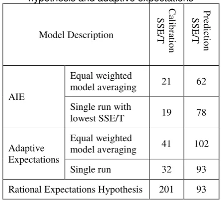
Table 2 compares the model variance from the calibration and prediction periods among the AIE, adaptive expectations and REH models. The calibration period is March 2000 to December 2006. The prediction period is March 2006 to June 2007. The REH requires no calibration as such. The predictive performance of AIE is better than the adaptive expectations and REH models. The programming code for the AIE model used to derive these results is available on a DVD as Appendix A to Bell (2009).

Table 2 Comparing the model variance (SSE/T) of the AIE model against the rational expectations

hypothesis and adaptive expectations

Model Description

C

alib

ra

tio

n

SSE

/T

P

re

d

ic

tio

n

SSE

/T

AIE

Equal weighted

model averaging 21 62

Single run with

lowest SSE/T 19 78

Adaptive Expectations

Equal weighted

model averaging 41 102

Single run 32 93

Rational Expectations Hypothesis 201 93

4 Conclusion and Implications

The interactive network component of the AIE model improves the temporal predictive performance of the model over the adaptive expectations model. Further, the result adds credibility to the network averaging as a technique to act as a proxy for networks that are unable to be measured or measured accurately. Additionally, the superior predictive performance of AIE over the

REH indicates that px is a superior model of choice

than the utility maximising agent and rational choice theory assumptions in REH for this D&B (2008) profit survey.

References

Arnsperger, C & Varoufakis, Y 2006, 'What Is

Neoclassical Economics? ' Post-autistic Economics

Bates, JM & Granger, CWJ 1969, 'The Combination of

Forecasts', Operational Research Quarterly, vol.

20, no. 4, pp. 451-68.

Beinhocker, ED 2006, Origin of Wealth: Evolution,

Complexity, and the Radical Remaking of Economics, Harvard Business School Press, Cambridge, Mass.

Bell, PW 2009, 'Adaptive Interactive Expectations: Dynamically Modelling Profit Expectations', University of Queensland.

Bowden, MP & McDonald, S 2006, 'The Effect of Social Interaction and Herd Behaviour on the

Formation of Agent Expectations', Computing in

Economics and Finance 2006, no. 178.

Camerer, C & Weber, M 1992, 'Recent developments in modeling preferences: Uncertainty and ambiguity ', Journal of Risk and Uncertainty, vol. 5, no. 4, pp. 325-70.

Choquet, G 1954, 'Theory of capacities', Annales

Institut Fourier, vol. 5, pp. 131-295.

D&B 2008, 'National Business Expectations Survey of business executives across Australia', viewed 20 February 2008,

<http://www.dnb.com.au/general/business_expectat ions/business_expectations.asp?id=pr_2007_1105& Link_Page=AUS>.

Dawid, H & Fagiolo, G 2008, 'Agent-based models for economics policy design: Introduction to the special

issue', Journal of Economic Behavior and

Organization, vol. 67, no. 2008, pp. 351-4. Eichberger, J, Kelsey, D & Schipper, BC 2009,

'Ambiguity and social interaction', Oxford

Economic Papers, vol. 61, no. 2, pp. 355-79. Ellsberg, D 1961, 'Risk, Ambiguity, and the Savage

Axioms ', The Quarterly Journal of Economics, vol.

75, no. 4, pp. 643-69.

Farmer, JD & Geanakoplos, J 2008, 'The Virtues and Vices of Equilibrium and the Future of Financial

Economics', Cowles Foundation, viewed 15 Feb.

2009, DOI Discussion Paper No. 1647,

<http://papers.ssrn.com/sol3/papers.cfm?abstract_id =1112664#>.

Flieth, B & Foster, J 2002, 'Interactive expectations',

Journal of Evolutionary Economics, vol. 12, no. 4, pp. 375-95.

Hicks, JR 1939, Value and capital, Oxford University

Press, London.

Kahneman, D 2002, 'Maps of Bounded Rationality: A Perspective on Intuitive Judgement and Choice', paper presented to Les Prix Nobel 2002, Stockholm,

<http://www.nobel.se/economics/laureates/2002/ka hnemann-lecture.pdf>.

Kahneman, D & Tversky, A 1979, 'Prospect Theory:

An analysis of decisions under risk', Econometrica,

vol. 47, no. 2, pp. 263-92.

Keen, S 2001, Debunking economics: the naked

emperor of the social sciences, Pluto Press, Annandale, N.S.W.

Keynes, JM 1937, 'The general theory of employment',

The Quarterly Journal of Economics, vol. 51 no. 2, pp. 209-23.

Knight, FH 1921, Risk, uncertainty and profit,

Houghton, New York.

Lucas Jr., RE 1986, 'Adaptive Behavior and Economic

Theory ', The Journal of Business, vol. 59, no. 4,

part 2, pp. S401-26.

Sargent, TJ 2008, 'Rational Expectations', in The

Concise Encyclopedia of Economics, Library of Economics and Liberty.

Savage, LJ 1954, The foundations of statistics, Wiley,

New York.

Tversky, A & Kahneman, D 1974, 'Judgment under uncertainty: Heuristics and biases', Science, vol. 185, pp. 1124-31.

Vercelli, A 2007, 'Rationality, learning and complexity: from the Homo economicus to the Homo sapiens',

in M Salzano & D Colander (eds), Complexity

Hints for Economic Policy Springer, Milan, New York.

Von Neumann, J & Morgenstern, O 1944, Theory of

games and economic behavior, Princeton University Press, Princeton.

Watts, DJ & Strogatz, SH 1998, 'Collective dynamics

of 'small-world' networks', Nature, vol. 393, pp.

440-2.

Wilensky, U 1999, NetLogo, Center for Connected

Learning and Computer-Based Modeling, Northwestern University, Evanston, IL, 30 May 2007, <http://ccl.northwestern.edu/netlogo/>.

— 2005, NetLogo Small Worlds model, Center for

Connected Learning and Computer-Based