ELMAN Neural Network with Modified Grey Wolf Optimizer for Enhanced Wind Speed Forecasting

(1)

http://dx.doi.org/10.4236/cs.2016.710255

How to cite this paper: Madhiarasan, M. and Deepa, S.N. (2016) ELMAN Neural Network with Modified Grey Wolf Opti-mizer for Enhanced Wind Speed Forecasting. Circuits and Systems, 7, 2975-2995.

http://dx.doi.org/10.4236/cs.2016.710255

ELMAN Neural Network with Modified Grey

Wolf Optimizer for Enhanced Wind Speed

Forecasting

M. Madhiarasan

*

, S. N. Deepa

#

Department of Electrical and Electronics Engineering, Anna University Regional Campus, Coimbatore, India

Received 28 April 2016; accepted 15 May 2016; published 16 August 2016

This work is licensed under the Creative Commons Attribution International License (CC BY).

http://creativecommons.org/licenses/by/4.0/

Abstract

The scope of this paper is to forecast wind speed. Wind speed, temperature, wind direction, relative humidity, precipitation of water content and air pressure are the main factors make the wind speed forecasting as a complex problem and neural network performance is mainly influenced by proper hidden layer neuron units. This paper proposes new criteria for appropriate hidden layer neuron unit’s determination and attempts a novel hybrid method in order to achieve enhanced wind speed forecasting. This paper proposes the following two main innovative contributions 1) both either over fitting or under fitting issues are avoided by means of the proposed new criteria based hidden layer neuron unit’s estimation. 2) ELMAN neural network is optimized through Modified Grey Wolf Optimizer (MGWO). The proposed hybrid method (ELMAN-MGWO) performance, effectiveness is confirmed by means of the comparison between Grey Wolf Optimizer (GWO), Adaptive Gbest-guided Gravitational Search Algorithm (GGSA), Artificial Bee Colony (ABC), Ant Colony Optimization (ACO), Cuckoo Search (CS), Particle Swarm Optimization (PSO), Evolution Strategy (ES), Genetic Algorithm (GA) algorithms, meanwhile proposed new criteria effectiveness and precise are verified compari-son with other existing selection criteria. Three real-time wind data sets are utilized in order to analysis the performance of the proposed approach. Simulation results demonstrate that the pro-posed hybrid method (ELMAN-MGWO) achieve the mean square error AVG ± STD of 4.1379e−11 ± 1.0567e−15, 6.3073e−11 ± 3.5708e−15 and 7.5840e−11 ± 1.1613e−14 respectively for evaluation on three real-time data sets. Hence, the proposed hybrid method is superior, precise, enhance wind speed forecasting than that of other existing methods and robust.

Keywords

ELMAN Neural Network, Modified Grey Wolf Optimizer, Hidden Layer Neuron Units, Forecasting, Wind Speed

(2)

1. Introduction

In recent year, wind energy is derived much more attention because of its special features such as inexhaustible, pollution free, free of availability, and renewable. Corresponding to the irregular and uncertain characteristics of wind speed, wind speed forecasting play a major role in wind farm and power system planning, scheduling, con-trolling and integration operation. Hence, the many researcher’s emphasis their research on the accurate wind speed forecasting in the literature: “Rough set theory and principal component analysis techniques incorporated ELMAN neural network based short-term wind speed forecasting performed by Yin, et al. [1]”. “Olaofe [2] presented Layered recurrent neural network (LRNN) forecasting model in order to forecast 5 day wind speed and wind pow-er”. “Hybrid wind speed forecasting approach combining empirical mode decomposition and ELMAN neural net-work is suggested by Wang, et al. [3]”. “Corne, et al. [4] carried out work on Evolved neural network based short- term wind speed forecasting”. “Cao, et al. [5] Analyzed wind speed forecasting by means of the ARIMA and recur-rent neural network based forecasting model; result proves superiority of the recurrecur-rent neural network than that of ARIMA”. “Junfang Li, et al. [6] performed one step ahead prediction of wind speed using ELMAN neural net-work”. “Madhiarasan and Deepa [7] performed different time scale forecasting of wind speed using six ANN (artifi-cial neural network) and performance analyzed with Coimbatore region three wind farm data sets”. “Madhiarasan and Deepa [8] presented wind speed prediction for different time scale horizon using Ensemble neural network”.

An Artificial neural network is an information processing structure designed by means interlinked elementary processing devices (neurons). Feed-forward neural network and feedback neural network are the general types of artificial neural network. The feedback neural network has a profound effect on the modeling nonlinear dynamic phenomena performance and its learning capacity. Determination of hidden layer units in artificial neural network is a crucial and challenging task, over fitting and under fitting problems is caused due to random choice of hidden layer units. Therefore, previous work in determining the hidden layer neuron units: “Arai [9] found the hidden units by means of TPHM”. “Jin-Yan Li, et al. [10] Searched optimal hidden units with the help of estimation theory”. “Proper hidden units for three and four layered feed-forward neural networks are defined by Tamura and Tateishi [11]”. “Kanellopoulas and Wilkinson [12] stated required amount hidden units”. “Osamu Fujita [13] determined feed forward neural network sufficient hidden units”. “Three layer binary neural network need hidden units are found based on set covering algorithm (SCA) by Zhaozhi Zhang, et al. [14]”. “Jinchuan Ke and Xinzhe Liu [15] pointed out neural network proper hidden units for stock price prediction”. “Shuxiang Xu and Ling Chen [16] de-scribed feed-forward neural network optimal hidden units”. “Multilayer perceptron network sufficient hidden units are defined by Stephen Trenn [17]”. “Katsunari Shibata and Yusuke Ikeda [18] stated large scale layered neural network sufficient hidden units and learning rate”. “David Hunter, et al. [19] Suggested the hidden units for multi-layer perceptron, bridged multimulti-layer perceptron and fully connected cascade”. “Gnana Sheela and Deepa [20] pointed out ELMAN neural network hidden units based on three input neurons”. “Guo Qian and Hao Yong [21] determined back propagation neural network hidden units”. “Madhiarasan and Deepa [22] Estimated improved back propagation network hidden units by means of novel criterion”. “Madhiarasan and Deepa [23] pointed out, recursive radial basis function network proper hidden layer neurons estimation based on new criteria”.

Optimizers have ability to give solution for a complex optimization problem and used to approximate the global optimum in order to improve the performance. Many researchers introduced new heuristic algorithms, some of the most familiar algorithms in the literature are: “Genetic Algorithm (GA) proposed by Holland [24]”, “Evolution Strategy (ES) pointed out by Ingo Rechenberg [25]”, “Particle Swarm Optimization (PSO) devel-oped by Kennedy and Eberhart [26]”, “Socha, K. and Blum [27] presented feed-forward neural network training by mean of the Ant Colony Optimization (ACO)”, “Karaboga and Basturk [28] carried out work on the Artifi-cial Bee Colony (ABC) for numerical function optimization”, “Yang and Deb [29] suggested Cuckoo search (CS) algorithm”, “Adaptive Gbest-guided Gravitational Search Algorithm (GGSA) proposed by Mirjalili and Lewis [30]”, “Mirjalili, et al. [31] developed Grey Wolf Optimizer (GWO)”.

This paper attempts to analyze the performance of ELMAN neural network based on the proposed 131 vari-ous criteria for proper hidden layer neurons units’ determination, Proposed new criteria estimate proper hidden neuron units in ELMAN neural network aid good forecasting result compared to other existing criteria and also proposed novel modified grey wolf optimizer (MGWO) to optimize the ELMAN neural network in order to im-prove the wind speed forecasting accuracy than earlier methods.

2. ELMAN Neural Network

(3)

ELMAN neural network comprises an input layer, hidden layer, recurrent link (feedback) layer and output layer. Recurrent layer placed in a network with one step delay of the hidden layer. ELMAN neural network is a recurrent network; recurrent links are added into the hidden layer as a feedback connection. “The ELMAN neural network dynamic characteristics are provided by internal connection; ELMAN neural network is superior to static feed- forward neural network because it does not require utilizing the states as training (or) input signal stated by Lin and Hung., Liu Hongmei, et al., Xiang Li, et al. [33]-[35]”. ELMAN neural network widely used for different applica-tion such as time series predicapplica-tion, modeling, control and speech recogniapplica-tion. Output is made from the hidden layer. The recurrent link layer stores the feedback and retains the memory. Hyperbolic tangent sigmoid activation func-tion is adopted for hidden layer and the purelin activafunc-tion funcfunc-tion is used for the output layer.

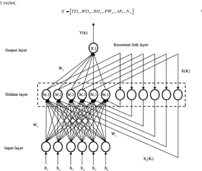
[image:3.595.114.528.352.704.2]

Proposed ELMAN neural network based wind speed forecasting model input layer is developed by means of the six input neurons, such as Temperature (TD_w), Wind Direction (WD_w), Relative Humidity (RH_w), Precipi-tation of Water content (PW_w), Air Pressure (AP_w) and Wind speed (N_w). Higher computational complexity and computation time are caused due to neural network with many hidden layers. Hence, the single hidden layer is used for neural network design. The output layer has a single output neuron (i.e.) forecast wind speed. The goal of the proposed new criteria is to choose exact hidden layer units to get the quick convergence and the best efficacy with the lowest mean square error. The architecture of the proposed ELMAN neural network based wind speed forecasting model is presented in Figure 1.

Figure 1 represented input and output target vector pairs are defined as follows.

(

X X1, 2,X3,X4,X5,X6:Y

)

= (Temperature, Wind Direction, Relative Humidity, Precipitation of Water

con-tent, Air Pressure and Wind speed: Forecast Wind speed).

(

X X1, 2,X3,X4,X5,X6:Y

)

=

(

TD WD RHw, w, w,PWw,AP Nw, w:Nfw

)

(1) Input vector,

[

_w, _w, _w, _w, _w, _w

]

X = TD WD RH PW AP N (2)

(4)

Output vector,

fw

Y = N _ (3)

Weight vectors of input to the hidden vector,

[

]

1 11, 12, , 1n, 21, 22, , 2n, 31, 32, , 3n, 41, 42, , 4n, 51, 52, , 5n, 61, 62, , 6n

W = W W W W W W W W W W W W W W W W W W (4)

Weight vectors of recurrent link layer vector,

[

]

2 21, 22, , 2n

W = W W W (5)

Weight vectors between context layer and input vector,

[

]

11 12 1 21 22 2 31 32 3 41 42 4

51 52 5 61 62 6

, , , , , , , , , , , , , , , ,

, , , , , , ,

c c c c n c c c n c c c n c c c n

c c c n c c c n

W W W W W W W W W W W W W

W W W W W W

=    

  (6)

ELMAN network inputs,

( )

(

c c

( )

1

(

1

)

X K =h W X K +W U K− (7)

ELMAN network output,

( )

(

2

( )

)

Y K = f W X K (8)

Input of recurrent link layer,

( )

(

1

)

c

X K = X K−

(9)

Let, N_fw is the forecast wind speed, W_c is connection weights between context layer and input layer, W₁ is connection weights between input layer and hidden layer, W₂ is connection weights between hidden layer and recurrent link layer, h

( )

⋅ is the hyperbolic tangent sigmoid activation function, f

( )

⋅ is purelin activation function.

For suggested ELMAN neural network each and every layer performs the individualistic calculations on receiv-ing information and the calculated results are passed to the succeedreceiv-ing layer and to end determines the network output this fact is observed from the Figure 1. Response to the current input depending on the previous inputs.

The neural network designing process plays a vital role in the network performance. A Proposed ELMAN network designed parameters include dimensions and epochs shown in Table 1. The input U K

(

−1

)

is passed through the hidden layer that multiplies weights (W₁) using hyperbolic tangent sigmoid activation function. Current input W U K₁

(

−1

)

plus previous state output W X_c _c

( )

K is helps the network to learn the function. The value of X K

( )

is passed through an output layer that multiplied with weights W₂ by means of the purelin activation function. For ELMAN neural network training process, the predecessor state information, gives back to the network. Training learned from the normalized data. Test for the stopping condition, the error coming to a very negligible value. Considered 131 various criteria are applied to ELMAN neural network one by one and verify the performance is accepted (or) not. The novel criteria are utilized to decide the proper hidden layer neuron units in ELMAN network construction and the presented approach is applied to forecast the wind speed.

3. Hidden Layer Neuron Units Estimation

[image:4.595.172.456.623.722.2]

The determination of hidden layer neuron units in a neural network frame is a tough task, odd choice of hidden

Table 1. Proposed ELMAN neural network designed parameters.

ELMAN Neural Network

Input neuron = 6

[

TD WD RH PW AP Nw, w, w, w, w, w

]

Number of hidden layer = 1

Output neuron = 1 Nfw

Number of epochs = 2000

(5)

layer neuron units cause either under fitting or over fitting issue. Several researchers have suggested lots of ap-proaches to select the hidden layer neuron units in neural networks. The apap-proaches can be categories into prun-ing and constructive approaches. “For prunprun-ing approach the neural network starts with bigger than the usual size and then removing superfluous neurons and weights, finally found the minimum neurons and weights, whereas on the constructive approach neural network begins with less than the usual size network and then additional hidden units are added to the neural network specified by Jin-Yan Li, et al., Mao and Guang-Bin Huang [10] [36]”. The artificial neural network with a small number of hidden neuron units may not have the enough ability to succeed the essentials namely error precision, network capacity and accuracy. The issue related to over fitting data is occurring due to over training process in the neural network design. Hence, determination of proper hid-den layer neuron units in artificial neural network construction is one of the great significance issue. Several re-searchers attempt to make the good network framework by tackling this problem. While on neural network modeling stage there is no other way to select the hidden layer neuron units without striving and verifying dur-ing the traindur-ing stage and calculatdur-ing the generalization error. If the hidden layer neuron units are large then hidden output connection weights become so small, learns easily and output neurons become unstable. If the hidden layer neuron units are small it may stuck in the local mini ma because the neural network learns very slowly so hidden units tends to unstable. Hence, determination of exact hidden layer neuron units is a significant censorious issue for neural network modeling. This article examines the appropriate determination of hidden layer neuron units for ELMAN neural network by means of the proposed new criteria. Features of the proposed criteria are as follows:

1) The proposed 131 various criteria are function of input neurons and noted to be justified based on conver-gence theorem.

2) Both either over fitting or under fitting problems are avoided.

3) To estimate exact hidden layer neuron units with minimal computational complexity.

All considered criteria were tested on ELMAN neural network to determine the neural network training and testing stage performance by statistical error. The implementation of the pointed out approach begins by adopt-ing the proposed criteria to ELMAN neural network. Followadopt-ing implementation stage train ELMAN neural network and calculate the mean square error (MSE). The network performance is calculated based on the mean square error; Equation (10) represents the mean square error formula. Criteria with the lowest minimal MSE (mean square error) are the best criteria for determination of hidden layer neuron units in ELMAN neural network.

Error Evaluation Measure is defined as follows:

(

)

2

1 1 MSE

N

i i i

O O

N =

′

=

∑

− (10)

where, O_i is forecast output, O_i′ is actual output, O_i is average actual output, N is the number of data sam-ples.

4. Modified Grey Wolf Optimizer (MGWO)

“GWO is recently employed by Mirjalili, et al. [31] in order to achieve improved performance by mean of search the global optimum”. In this paper modified grey wolf optimizer is proposing in ELMAN neural net-works for wind speed forecasting. Modified grey wolf optimizer proves with improved exploration and exploita-tion than that of GWO and other evoluexploita-tionary strategies. Modified grey wolf optimizer replicates the social lea-dership and prey hunting behavior of grey wolves. The population is split into four groups alpha (

α

), beta (

β

), gamma (γ) and lambda (λ) for the proposed MGWO.

The favorable area of the search space attains by the wolves λ based on the direction of the first three fittest wolves such as alpha (

α

), beta (

β

) and gamma (γ). The wolves revise their position around

α

,

β

and γ during a course of optimization stage are given as below:

( )

p i i worst i

= ⋅ − −

D G P P P (11)

(

i+ =1

)

( )

i − ⋅

P P H D (12)

where, i—Current Epoch, P—Position vector of the grey wolf, P_worst—Position vector of the worst grey wolf, p

(6)

1 2

= ⋅ −

H u v u, G= ⋅2 v₂ where, u—Set to linearly decreased from 2 to 0 during the course of epochs, v₁ & v₂—Random vector between 0 & 1.

The rest of the candidates (λ wolves) revise their position based on the first three fitness solution such as

α

,

β

and γ are described as follows:

1 worst

α = ⋅ α− −

D G P P P (13)

2 worst

β = ⋅ β − −

D G P P P

(14)

3 worst

γ = ⋅ γ− −

D G P P P (15)

( )

1= α− 1⋅ α

P P H D

(16)

( )

2 = β− 2⋅ β

P P H D

(17)

( )

3 = γ− 3⋅ γ

P P H D

(18)

(

) (

1 2 3

)

1

3 i+ = P +P +P

P (19)

where, P_α—Position of the first best solution (

α

), P_β—Position of the second best solution (

β

), P_γ —Posi- tion of the third best solution (γ), P—Current position, i—Number of epochs, H H₁, ₂&H₃—Random vectors.

The relative distance between the present solution and

α

,

β

, γ respectively, are estimated by means of the Equations (13)-(15). The eventual position of the present solution is estimated after the distance computa-tions are expressed in Equacomputa-tions (16)-(19). The coefficient vectors are playing a key role for better exploration and exploitation; if G>1 it promoted exploration meanwhile H <1 exploitation is emphases. Modified Grey Wolf Optimization (MGWO) achieves better convergence than that of GWO by means of the inclusion of the worst position.

Steps involved in MGWO Algorithm are as follows:

Step1: Based on the variables upper and lower bounds randomly initialize a population of wolves. Step2: Compute each wolf corresponding fitness value.

Step3: Store the first three best wolves as

α

,

β

, γ respectively.

Step4: Update the rest of the search agents (λ wolves) position by means of Equations (11)-(19). Step5: Update variables such as u, H and G.

Step6: If stopping criteria is not satisfied go to Step2. Step7: Record

α

position as the best global optimum.

Proposed novel Modified Grey Wolf Optimizer (MGWO) algorithm flow chart is shown inFigure 2.

5. ELMAN Neural Network with MGWO

The highest forecasting accuracy is provided by means of the optimization techniques. Therefore, novel mod-ified grey wolf optimizer (MGWO) is attempting to optimize the ELMAN neural network for wind speed fore-casting application. Figure 3 depicts the structure of the ELMAN neural network optimization by MGWO. Mean square error (MSE) is generally used performance measure for evaluation of forecasting accuracy. MSE computed based on the Equation (10), the lowest mean square error indicates the improved forecasting accuracy. Hence, the minimization of MSE is used as an objective function for the proposed MGWO algorithm. The weights of the ELMAN neural network are provided by means of the MGWO algorithm, MGWO perform the minimization MSE based on changing weights (i.e. weight optimization). Weights changing of wolves are high-ly influenced based on the

α

wolf, the best weight are searched by means of the MGWO in order to improve the convergence, accuracy and minimizes ELMAN neural network error.

6. Result Analysis and Discussion

6.1. Data Resources and Simulation Platform

(7)

[image:7.595.85.540.70.717.2]

Figure 2. MGWO algorithm flow chart.

(8)

Atmospheric Administration, United States from January 1994 to December 2014. Data set 2 and Data set 3 are observed from Suzlon Energy Private Limited from January 2010 to December 2014 with different wind mill height. All data set contains 100,000 number of data samples. The neural network based wind speed forecasting approach involves the designing, training and testing stages. Exact modeling of neural network is difficult and a tough task. The gathered input attributes used for ELMAN neural network are real-time data therefore, scaling procedure is used up to avoid the training process issues such as massive esteemed input data incline to minimize the impact of little value input data. Therefore, the min-max scaling method is used to scale the variable range of real-time data within the range of 0 to 1; scaling is computed based on the Equation (20). The scaling process helps to improve the numerical computational accuracy, so ELMAN neural network model accuracy is also enhanced.

Scaled input,

(

)

_ min

_ max _ min _ min _ max _ min

a a

a t t t

a a

X X

X X X X

X X

 − 

′ =_ _ ′ − ′ + ′

−

  (20)

where, X_a is actual input data, X_a_{_ min} is minimum of actual input data, X_a_{_ max} is maximum of actual input data, X_t′_{_ min} is the minimum of the target, X_t′_{_ max} is the maximum of the target.

The proposed ELMAN neural network is established by three real-time data sets; each acquired real-time data sets consists up of 100,000 numbers of data samples. The collected 100,000 real-time data are classified as training and testing. The collected 70% of data (70,000) are utilized for neural network training phase and 30% of the gathered data (30,000) are utilized for the testing phase of the network. Proposed neural network design and all algorithms are tested in MATLAB and simulate on an Acer computer with Pentium (R) Dual Core pro-cessor running at 2.30 GHZ with 2 GB of RAM.

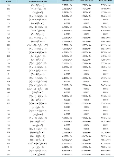
6.2. Proposed Criteria Based Estimation of Hidden Layer Neuron Units

The issues related to the proper determination of hidden layer neuron units for a specific problem are to be cho-sen. The existing strategies utilizes trial and error rule for deciding neural networks hidden layer neuron units. This begins the network with less than the usual size of hidden layer neuron units and additional hidden neurons are included in the N_h. Limitations are there are no assurance of deciding the hidden layer neuron units and it consumes much time. Therefore, propose the new 131 criteria as a function of input neurons to determine the hidden layer neuron units in neural networks. The appropriate hidden layer neuron units in hidden layer are de-termined based on the best the lowest minimal error. Three real-time data sets are used for performance analysis of considered 131 various criteria for determination of the hidden layer neuron units in ELMAN neural network based on the mean square error are established in Table 2. Results obtained with the three real-time data sets proved that the proposed criteria un =

(

5n+2

) (

n−5

)

 based hidden layer neuron unit’s estimation in

ELMAN neural network achieved minimal mean square error than other considered criteria. Therefore, the pro-posed criteria to improve the effectiveness and accuracy for wind speed forecasting.

Justification for the Chosen Criteria

Justification for determination of hidden layer neuron units is commenced by means of the convergence theo-rem discussion in the Appendix. Lemma 1 confirms the convergence of the chosen criteria.

Lemma 1:

The sequence un =

(

5n+2

) (

n−5

)

 is converging and un≥0.

The sequence tends to have a finite limit l, if there exists constant ε >0 such thatu_n− <l ε, then lim n n→∞u =l. Proof:

Lemma 1 based proof defined as follows.

Regarding to convergence theorem, the selected value (or) sequence converges to a finite limit value.

(

5 2

)

5 n n u n + =

− , (21)

(

)

5 2

lim lim 5

5 5 1 n n n n n n n n →∞ →∞  ₊    + _ _ = = −  ₋     

(9)

[image:9.595.89.533.111.723.2]

Table 2.ELMAN neural network statistical analysis of various criteria for determination of hidden layer neuron units.

Hidden neuron Units

Examined Criteria for determination of

hidden neuron Units Data set1 MSE Data set2 MSE Data set3 MSE

33

(

6n−3

) (

n−5

)

7.5783e−04 7.5783e−04 7.5783e−04 130

(

10(n+7)

)

(n−5) 3.3291e−04 3.4342e−04 3.9400e−04 12

( ) (

2n n−5

)

9.5408e−04 1.1030e−03 1.1380e−03 74

(

8(n+3)+2

)

(n−5) 8.0641e−04 8.4120e−04 8.6321e−04

119

(

8(n+9)−1

)

(n−5) 0.0016 0.0019 0.0020

23

(

4n−1

) (

n−5

)

0.0011 0.0012 0.0013

89

(

9(n+4)−1

)

(n−5) 6.7827e−04 6.9402e−04 7.0476e−04 62

(

10n+2

) (

n−5

)

8.8395e−04 8.9911e−04 9.1059e−04

35

(

5n+5

) (

n−5

)

0.0018 0.0021 0.0022

124

(

8(n+9)+4

)

(n−5) 3.1087e−04 3.4500e−04 3.6651e−04 50

(

8n+2

) (

n−5

)

5.0931e−04 5.3125e−04 5.5697e−04

116

(

2

)

(

2

)

3 n +2 +2 n −35 3.7581e−04 3.9733e−04 4.1111e−04 85

(

9(n+3)+4

)

(n−5) 4.6975e−04 4.8956e−04 4.9577e−04 28

(

3(n+3)+1

)

(n−5) 4.7696e−04 4.9023e−04 5.0789e−04

106

(

2

) (

2

)

3n −2 n −35 5.9167e−04 6.0045e−04 6.1072e−04 57

(

9n+3

) (

n−5

)

4.7917e−04 4.8232e−04 5.2004e−04

70

(

2

)

(

2

)

2 n −1 n −35 7.1026e−04 7.5088e−04 7.7720e−04 92

(

9(n+4)+2

)

(n−5) 5.0730e−04 5.6589e−04 5.8301e−04

111

(

2

)

(

2

)

3 n +1 n −35 0.0010 0.0011 0.0012

8

(

2n−4

) (

n−5

)

0.0013 0.0016 0.0019

46

(

4(n+5)+2

)

(n−5) 6.4050e−04 6.7652e−04 6.9137e−04

128

(

2

)

(

2

)

4 n −4 n −35 0.0016 0.0018 0.0019

76

(

2

)

(

2

)

2 n +2 n −35 7.1067e−04 7.3284e−04 7.6471e−04

131

(

2

)

(

2

)

3 n +7 +2 n −35 0.0011 0.0013 0.0015

60

( ) (

10n n−5

)

0.0013 0.0015 0.0016 51

(

7(n+ +1) 2

)

(n−5) 9.1476e−04 9.4678e−04 9.7125e−04

26

(

4n+2

) (

n−5

)

0.0016 0.0018 0.0019

102

(

8(n+7)−2

)

(n−5) 7.2283e−04 7.5392e−04 7.7487e−04

11

(

n+5

) (

n−5

)

0.0013 0.0014 0.0016

94

(

7(n+7)+3

)

(n−5) 0.0012 0.0014 0.0015

36

( ) (

6n n−5

)

0.0012 0.0015 0.0018 87

(

9(n+4)−3

)

(n−5) 7.6306e−04 7.8540e−04 7.9121e−04 55

(

5(n+5)

)

(n−5) 4.2964e−04 4.6008e−04 4.8257e−04 24

( ) (

4n n−5

)

0.0023 0.0026 0.0029

80

(

2

)

(

2

)

2 n +4 n −35 0.0017 0.0018 0.0019

108

(

9(n+6)

)

(n−5) 2.9367e−04 3.1955e−04 3.4276e−04 16

(

4(n−2)

)

(n−5) 6.1773e−04 6.9457e−04 7.0121e−04 72

(

8(n+3)

)

(n−5) 6.7910e−04 6.9122e−04 7.0011e−04

121

(

2

)

( )

3 n +4 +1 n−5 8.6702e−04 8.9780e−04 9.2144e−04

7

(

n+1

) (

n−5

)

6.8433e−04 6.9510e−04 7.0281e−04

(10)

Continued

110

(

9(n+6)+2

)

(n−5) 0.0011 0.0012 0.0013

14

(

3(n−2)+2

)

(n−5) 0.0013 0.0016 0.0018

84

(

2

)

(

2

)

2 n +6 n −35 4.5795e−04 4.7541e−04 4.9123e−04

47

(

7n+5

) (

n−5

)

0.0013 0.0015 0.0017

52

(

8n+4

) (

n−5

)

5.6372e−04 5.8620e−04 6.1781e−04 129 9

(

(n+8)+3

)

(n−5) 6.9995e−04 7.2241e−04 7.5599e−04 67

(

7(n+4)−3

)

(n−5) 8.4212e−04 8.5627e−04 8.7560e−04

120

(

10(n+6)

)

(n−5) 0.0017 0.0018 0.0021

34

(

2

) (

2

)

2 35

n − n − 0.0011 0.0012 0.0013

65

(

9(n+1)

)

(n−5) 0.0010 0.0011 0.0013

41

(

5(n+2)+1

)

(n−5) 9.7246e−04 9.8904e−04 1.0031e−04

2

(

n−4

) (

n−5

)

3.1075e−04 3.4312e−04 3.5422e−04

105

(

7(n+9)

)

(n−5) 0.0010 0.0012 0.0013

78

(

8(n+4)−2

)

(n−5) 7.4818e−04 7.6578e−04 7.8117e−04

43

(

6n+7

) (

n−5

)

0.0014 0.0017 0.0019

27

(

4(n+ −1) 1

)

(n−5) 4.3249e−04 4.6417e−04 4.9710e−04 112

(

8(n+8)

)

(n−5) 4.1333e−04 4.3266e−04 4.6782e−04

56

(

7(n+2)

)

(n−5) 0.0011 0.0013 0.0014

81

(

9(n+3)

)

(n−5) 2.4019e−04 2.6387e−04 2.7023e−04 9

(

n+3

) (

n−5

)

6.7128e−04 6.8430e−04 6.9281e−04

73

(

2

) (

2

)

2n +1 n −35 0.0010 0.0012 0.0013

38 (6n+2) (n−5) 0.0020 0.0021 0.0023

123

(

2

)

(

2

)

3 n +5 n −35 5.0271e−04 5.4437e−04 5.7759e−04 63

(

7(n+3)

)

(n−5) 7.8566e−04 7.9623e−04 8.0146e−04

25

(

3n+7

) (

n−5

)

0.0024 0.0027 0.0030

100

(

7(n+8)+2

)

(n−5) 8.1476e−04 8.2761e−04 8.5690e−04

96

(

8(n+6)

)

(n−5) 0.0032 0.0035 0.0036

18

(

2n+6

) (

n−5

)

9.7457e−04 1.0232e−03 1.3615e−03

40

(

4(n+4)

)

(n−5) 0.0022 0.0025 0.0027

117

(

9(n+7)

)

(n−5) 7.9870e−04 8.0045e−04 8.2458e−04

3

(

2n−9

) (

n−5

)

0.0020 0.0024 0.0026

69

(

7(n+4)−1

)

(n−5) 5.0433e−04 5.3025e−04 5.6781e−04

88

(

8(n+5)

)

(n−5) 0.0013 0.0015 0.0017

104

(

8(n+7)

)

(n−5) 4.8877e−04 4.9761e−04 5.0780e−04 20

(

4(n−1)

)

(n−5) 6.2597e−04 6.5780e−04 6.9541e−04 77

(

9(n+2)+5

)

(n−5) 5.1210e−04 5.4209e−04 5.8122e−04 54

( ) (

9n n−5

)

3.9739e−04 4.2351.e−04 4.5028e−04

127

(

2

)

(

2

)

3 n +6 +1 n −35 2.9093e−04 3.0314e−04 3.2410e−04

10

(

2(n−1)

)

(n−5) 0.0011 0.0012 0.0013

58

(

10n−2

) (

n−5

)

0.0014 0.0016 0.0017

114

(

2

)

( )

3n +2 n−5 9.2745e−04 9.5492e−04 9.7560e−04

39

(

7n−3

) (

n−5

)

0.0014 0.0016 0.0018

122

(

8(n+9)+2

)

(n−5) 3.5541e−04 3.8012e−04 3.9956e−04

(11)

Continued

13

(

3n−5

) (

n−5

)

1.9842e−04 2.5013e−04 2.8917e−04 45

(

5(n+3)

)

(n−5) 5.7558e−04 5.8689e−04 6.1358e−04

29

(

6n−7

) (

n−5

)

0.0013 0.0015 0.0017

109

(

8(n+7)+5

)

(n−5) 2.6082e−04 2.7920e−04 2.9215e−04

6

( ) (

n n−5

)

0.0018 0.0020 0.0021

53

(

6(n+3)−1

)

(n−5) 0.0015 0.0017 0.0018

118

(

2

)

(

2

)

3 n +3 +1 n −35 0.0011 0.0012 0.0013

37

(

2

) (

2

)

1 35

n + n − 0.0015 0.0017 0.0019

126

(

9(n+8)

)

(n−5) 7.9942e−04 8.0923e−04 8.2031e−04 59

(

9n+5

) (

n−5

)

8.3566e−04 8.6168e−04 8.9610e−04

17

(

3n−1

) (

n−5

)

0.0015 0.0019 0.0020

83

(

8(n+4)+3

)

(n−5) 6.8054e−04 6.8994e−04 6.9461e−04 101

(

9(n+5)+2

)

(n−5) 4.0597e−04 4.3111e−04 4.6787e−04 93

(

8(n+5)+5

)

(n−5) 5.6662e−04 5.7554e−04 5.8530e−04

66

(

2

)

(

2

)

2 n −3 n −35 8.2555e−04 8.6592e−04 8.8509e−04 42

( ) (

7n n−5

)

4.8333e−04 4.9612e−04 5.1211e−04 75

(

7(n+4)+4

)

(n−5) 4.1790e−04 4.5239e−04 4.7854e−04 30

( ) (

5n n−5

)

7.7837e−04 7.9846e−04 8.3071e−04

95

(

2

)

(

2

)

2 n +9 +5 n −35 0.0015 0.0016 0.0017

79

(

7(n+5)+2

)

(n−5) 0.0012 0.0013 0.0015

86

(

2

)

(

2

)

2 n +7 n −35 2.2093e−04 2.5033e−04 2.7311e−04 22

(

5n−8

) (

n−5

)

5.5179e−04 5.9641e−04 6.0247e−04

64

(

8(n+2)

)

(n−5) 0.0025 0.0026 0.0028

4

(

n−2

) (

n−5

)

0.0012 0.0015 0.0018

97

(

2

)

(

2

)

2 n +9 +7 n −35 6.4348e−04 6.6046e−04 6.8751e−04

82

(

2

)

(

2

)

2 n +5 n −35 5.0672e−04 5.5223e−04 5.8548e−04 113

(

9(n+6)+5

)

(n−5) 1.9020e−04 1.9941e−04 2.0102e−04

90

(

2

)

(

2

)

2 n +9 n −35 0.0010 0.0011 0.0012

48

( ) (

8n n−5

)

0.0010 0.0012 0.0013

71

(

9(n+2)−1

)

(n−5) 0.0011 0.0012 0.0013

19

(

3n+1

) (

n−5

)

8.5313e−04 8.9130e−04 9.3103e−04 21

(

3(n+1)

)

(n−5) 6.1903e−04 6.6278e−04 6.8543e−04 103

(

7(n+9)−2

)

(n−5) 9.4000e−04 9.6203e−04 9.9055e−04 32

(

5n+2

) (

n−5

)

2.9538e−05 3.6592e−05 4.2505e−05

5

(

2(n−3)−1

)

(n−5) 0.0020 0.0023 0.0025

91

(

7(n+7)

)

(n−5) 0.0012 0.0014 0.0015

107

(

9(n+6)−1

)

(n−5) 6.4686e−04 6.7332e−04 6.8697e−04 44

(

4(n+5)

)

(n−5) 5.0210e−04 5.4579e−04 5.8435e−04

125

(

2

)

(

2

)

3 n +5 +2 n −35 4.1907e−04 4.3321e−04 4.5548e−04

15

(

n+9

) (

n−5

)

4.3777e−04 4.9050e−04 5.4307e−04

98

(

7(n+8)

)

(n−5) 8.8330e−04 8.9654e−04 9.1113e−04

31

(

3(n+4)+1

)

(n−5) 0.0027 0.0029 0.0031

1

(

2(n−5)−1

)

(n−5) 9.4851e−04 9.7128e−04 9.8429e−04

115

(

8(n+8)+3

)

(n−5) 0.0011 0.0012 0.0013

(12)

Here 5 is the limit value of the chosen sequence as lim

n→∞. Hence, the examine sequence tends to have a finite limit so it is convergent sequence; where n is the input neuron units.

Experimental results confirm that the chosen criteria

(

5n+2

) (

n−5

)

which possess 32 hidden layer neuron units in ELMAN neural network achieved the lowest mean square error (MSE) value 2.9538e−05, 3.6592e−05 and 4.2505e−05 for wind speed forecasting tested with three real-time data sets respectively. Hence, criteria

(

5n+2

) (

n−5

)

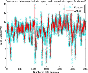
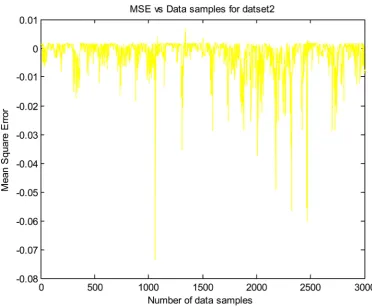
determined as the best solution for determination of hidden layer neuron units in neural net-work model. The proposed ELMAN neural netnet-work based wind speed forecasting revealed that the forecast wind speed is in supreme compatibility with actual wind speed, it can be noticed from experimental results.

Figures 4-6 show the comparison between actual wind speed and forecast wind speed obtained from the pro-posed new criteria based ELMAN neural network for the data sets1, data sets2 and data sets3, respectively. Wind speed forecasting on three real-time data sets using new criteria based ELMAN neural network make con-sistent results with precise match with actual wind speed; it is easy to notice from Figures 4-6. Figures 7-9depict the mean square error vs. number of data samples obtained from the proposed new criteria based ELMAN neural network for the data sets1, data sets2 and data sets3, respectively. Based on the experiments on three real-time data sets, proposed criteria

(

5n+2

) (

n−5

)

is consistent with the result of lower mean square error, it is inferred fromFigures 7-9. For clarity of the graph only part of result with 3000 data samples is shown. The Merits of the presented method are very effective, minimal error and easy implementation for wind speed forecasting.

Comparison with Exiting Criteria

Analysis proposed criteria effectiveness compared with the result of other existing criteria based hidden layer neuron unit’s estimation in ELMAN neural network for wind speed forecasting is presented in Table 3. The

[image:12.595.135.491.409.708.2]

Table 3shows, the importances of the proposed criteria get the lower mean square error. Obviously, the pro-posed criteria

(

5n+2

) (

n−5

)

aid better winds speed forecasting performance in terms of reduced errors. The comparison confirmed that the attempting new criteria have the lowest mean square error than other existing criteria.

(13)

[image:13.595.129.490.83.378.2]

Figure 5. Comparison between actual wind speed and forecast wind speed for data set2.

[image:13.595.131.495.399.700.2]

(14)

[image:14.595.125.500.83.390.2]

Figure 7. MSE vs. data samples for data set1.

[image:14.595.125.498.400.708.2]

(15)

[image:15.595.127.503.79.382.2]

Figure 9.MSE vs. data samples for data set3.

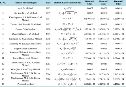
Table 3.Comparative analysis of proposed method performance with earlier various methodologies.

S. No. Various Methodologies Year Hidden Layer Neuron Units Data set1 MSE

Data set2 MSE

Data set3 MSE

1 Arai, M Method 1993 2 3n

h

N = 0.0025 0.0026 0.0028

2 Jin-Yan Li et al. Method 1995 Nh=

(

1 8+ n−1

)

2 0.0012 0.0015 0.0018

3 Kanellopoulas, I & Wilkinson, G, G

Method 1997 Nh= ∗N 2 9.5408e−04 1.1030e−03 1.1380e−03

4 Tamura, S & Tateishi, M Method 1997 Nh= −N 1 0.0020 0.0023 0.0025

5 Osamu Fujita Method 1998

(

( )0

)

log / log

h v

N =K P Z C S 5.1210e−04 5.4209e−04 5.8122e−04

6 Zhaozhi Zhang et al. Method 2003 2n

(

1

)

h

N = n+ 6.7128e−04 6.8430e−04 6.9281e−04

7 Jinchauan Ke & Xinzhe Lie Method 2008 Nh=

(

Nin+ Np L

)

7.9870e−04 8.0045e−04 8.2458e−04

8 Shuxiang Xu & Ling Chen Method 2008 Nh=Cf

(

N (dlogN)

)

1 2 0.0013 0.0015 0.0017 9 Stephen Trenn Approach 2008 Nh= + −

(

n n0 1 2

)

0.0020 0.0024 0.0026

10 Katsunari Shibata & Yusuke Ikeda

Method 2009

( )i ( )o h

N = N N 3.1075e−04 3.4312e−04 3.5422e−04

11 David Hunter et al. Method 2012 2n 1 h

N = − 7.8566e−04 7.9623e−04 8.0146e−04

12 Gnana Sheela, K & S, N, Deepa

Method 2013

(

) (

)

2 2

4 3 8

h

N = n + n − 0.0020 0.0023 0.0025

13 Gue Qian & Hao Yong Method 2013 Nh= n+ +m a 0.0012 0.0015 0.0018

14 Madhiarasan, M & S, N, Deepa

Method 2016 Nh=

(

8n−4

) (

n−4

)

5.0210e−04 5.4579e−04 5.8435e−04 15 Madhiarasan, M & S, N, Deepa

Method 2016

(

)

(

)

2 2

2 5 3 1 8

h

N = n + + n − 1.9842e−04 2.5013e−04 2.8917e−04

[image:15.595.94.540.417.723.2]

(16)

6.3. Proposed Modified Grey Wolf Optimizer Based ELMAN Neural Network and

Comparison with Existing Algorithms

Chosen new criteria based ELMAN neural network possesses 6 input neuron units, single hidden layer with 32 hidden layer neuron units and single output optimized by means of the proposed modified grey wolf optimizer.

[image:16.595.87.537.195.720.2]

For substantiation of the proposed algorithm, the results are compared with some of the existing Meta heuris-tic algorithms. A similar wind speed forecasting and objective function is used for ELMAN neural network with the Meta heuristic algorithm in Table 4. Due to the stochastic nature of Meta heuristic algorithm, the three

Table 4. Compared algorithms initial parameters.

Algorithms Parameters Parametric Values

MGWO

Population size u

Maximum number of generations

100

Linearly decreased from 2 to 0 300

GWO

Population size a

100

Linearly decreased from 2 to 0 300 GGSA Population size 1 c′ 2 c′ 0 G α

100

(

3 3

)

2t T 2

− +

(

3 3

)

2t T

1 20 300 CS Population size α ρ

100 0.3 300 ABC Population size Limit

100 20 300

ACO

Population size Initial pheromone (τ) Pheromone update constant (Q)

Pheromone constant (q)

Global pheromone decay rate (pg)

Local pheromone decay rate(p1)

Pheromone sensitivity (α) Visibility sensitivity (β) Maximum number of generations

100 1e−07 30 1 0.8 0.5 1 5 300 PSO Population size

1& 2

C C

100 1.5 300 ES Population size λ σ

100 10 1 300 GA Type Selection Crossover Mutation Population size Maximum number of generations

Real coded Roulette wheel Single point (probability = 1)

Uniform (probability = 0.1) 100

(17)

[image:17.595.88.534.393.724.2]

different wind data sets are solved over 20 runs using each algorithm in order to generate the statistical results. Statistical results are depicted in Table 5 in the form of the average and standard deviation of the MSE, the lowest average and standard deviation of MSE indicate the superior performance, proposed hybrid method (ELMAN-MGWO) achieve average and standard deviation of the MSE for three real-time data sets are 4.1379e−11 ± 1.0567e−15, 6.3073e−11 ± 3.5708e−15 and 7.5840e−11 ± 1.1613e−14 respectively. From the

Table 5, it can be noticed that the proposed modified grey wolf optimizer based ELMAN neural network obtain the minimal mean square error for three real-time wind data sets than those obtained with other existing algo-rithms. Therefore, the proposed modified grey wolf optimizer based ELMAN neural network not only produces improved forecasting accuracy with minimal mean square error, but also improves the convergence, stability and reduce the computation time.

7. Conclusion

In this paper, a novel hybrid method (ELMAN-MGWO) is proposed for wind speed forecasting. Firstly, proper hidden layer neuron unit is estimated based on the proposed new criteria and suggested criteria are validated based on the convergence theorem. Based on the least mean square error

(

5n+2

) (

n−5

)

is identified as the best criteria. ELMAN neural network with the best criteria obtain MSE of 2.9538e−05, 3.6592e−05 and 4.2505e−05 experimentation on three real-time data sets respectively. Secondly, the modified grey wolf optimizer is adopted to optimize the ELMAN neural network. Thirdly, investigating the performance of the proposed hybrid method by means of the three real-time data sets and effectiveness is evaluated based on the performance metric and computed error. Hybrid method (ELMAN-MGWO) obtains mean square error average and standard deviation as 4.1379e−11 ± 1.0567e−15, 6.3073e−11 ± 3.5708e−15 and 7.5840e−11 ± 1.1613e−14 respectively for validation on three real-time data sets. Finally, comparative analysis is performed in order to demonstrate that the proposed new criteria based hybrid method make faster convergence, robust, accurate and effective for wind speed forecast-ing. Hence, the proposed method is useful for wind farm and power system operation and control.

Table 5.Statistical results comparison.

Data sets Algorithms _{AVG ± STD}MSE

Data set1 GA-ELMAN ES-ELMAN PSO-ELMAN ACO-ELMAN ABC-ELMAN CS-ELMAN GGSA-ELMAN GWO-ELMAN MGWO-ELMAN

8.1107e−07 ± 3.0232e−03 2.7001e−07 ± 3.1831e−04 3.1518e−08 ± 7.8981e−07 5.8667e−07 ± 7.1113e−03 7.7032e−09 ± 3.7518e−06 6.7807e−09 ± 9.0901e−07 7.0563e−09 ± 9.9493e−06 2.2192e−10 ± 3.8892e−10

4.1379e−11 ± 1.0567e−15

6.3073e−11 ± 3.5708e−15

(18)

Acknowledgements

The authors gratefully acknowledge National Oceanic and Atmospheric Administration, United States and Suz-lon Energy Private Limited for the provision of data resources. Mr. M. Madhiarasan was supported by the Rajiv Gandhi National Fellowship (F1-17.1/2015-16/RGNF-2015-17-SC-TAM-682/(SA-III/Website)).

References

[1] Yin, D.-Y., Sheng, Y.-F., Jiang, M.-J., Li, Y.-S. and Xie, Q.-T. (2014) Short-Term Wind Speed Forecasting Using El-man Neural Network Based on Rough Set Theory and Principal Components Analysis. Power System Protection and

Control, 42, 46-51.

[2] Olaofe, Z.O. (2014) A 5-Day Wind Speed & Power Forecasts Using a Layer Recurrent Neural Network (LRNN).

Sus-tainable Energy Technologies and Assessments, 6, 1-24. http://dx.doi.org/10.1016/j.seta.2013.12.001

[3] Wang, J., Zhang, W., Li, Y., Wang, J. and Dang, Z. (2014) Forecasting Wind Speed Using Empirical Mode Decompo-sition and Elman Neural Network. Applied Soft Computing, 23, 452-459. http://dx.doi.org/10.1016/j.asoc.2014.06.027 [4] Corne, D.W., Reynolds, A.P., Galloway, S., Owens, E.H. and Peacock, A.D. (2013) Short Term Wind Speed

Forecast-ing with Evolved Neural Networks. Proceedings of the 2013 Genetic and Evolutionary Computation Conference

Companion, Amsterdam, 6-10July 2013, 1521-1528. http://dx.doi.org/10.1145/2464576.2482731

[5] Cao, Q., Ewing, B.T. and Thompson, M.A. (2012) Forecasting Wind Speed with Recurrent Neural Networks.

Euro-pean Journal of Operational Research, 221, 148-154. http://dx.doi.org/10.1016/j.ejor.2012.02.042

[6] Li, J., Zhang, B., Mao, C., Xie, G.L., Li, Y. and Lu, J. (2010) Wind Speed Prediction Based on the Elman Recursion Neural Networks. The 2010 International Conference on Modelling, Identification and Control (ICMIC), Okayama, 17-19 July 2010, 728-732.

[7] Madhiarasan, M. and Deepa, S.N. (2016) Performance Investigation of Six Artificial Neural Networks for Different Time Scale Wind Speed Forecasting in Three Wind Farms of Coimbatore Region. International Journal of Innovation

and Scientific Research, 23, 380-411.

[8] Madhiarasan, M. and Deepa, S.N. (2016) Application of Ensemble Neural Networks for Different Time Scale Wind Speed Prediction. International Journal of Innovative Research in Computer and Communication Engineering, 4, 9610-9617.

[9] Arai, M. (1993) Bounds on the Number of Hidden Units in Binary-Valued Three-Layer Neural Networks. Neural

Networks, 6, 855-860. http://dx.doi.org/10.1016/S0893-6080(05)80130-3

[10] Li, J.-Y., Chow, T.W.S. and Yu, Y.-L. (1995) The Estimation Theory and Optimization Algorithm for the Number of Hidden Units in the Higher-Order Feed Forward Neural Network. Proceeding IEEE International Conference on

Neural Networks, 3, 1229-1233. http://dx.doi.org/10.1109/ICNN.1995.487330

[11] Tamura, S. and Tateishi, M. (1997) Capabilities of a Four-Layered Feed Forward Neural Network: Four Layer versus Three. IEEE Transaction on Neural Network, 8, 251-255. http://dx.doi.org/10.1109/72.557662

[12] Kanellopoulas, I. and Wilkinson, G.G. (1997) Strategies and Best Practice for Neural Network Image Classification.

International Journal of Remote Sensing, 18, 711-725. http://dx.doi.org/10.1080/014311697218719

[13] Fujita, O. (1998) Statistical Estimation of the Number of Hidden Units for Feed Forward Neural Network. Neural

Network, 11, 851-859. http://dx.doi.org/10.1016/S0893-6080(98)00043-4

[14] Zhang, Z.Z., Ma, X.M. and Yang, Y.X. (2003) Bounds on the Number of Hidden Neurons in Three-Layer Binary Neural Networks. Neural Network, 16, 995-1002. http://dx.doi.org/10.1016/S0893-6080(03)00006-6

[15] Ke, J.C. and Liu, X.Z. (2008) Empirical Analysis of Optimal Hidden Neurons in Neural Network Modeling for Stock Prediction. IEEE Pacific-Asia Workshop on Computational Intelligence and Industrial Application, 2, 828-832. http://dx.doi.org/10.1109/PACIIA.2008.363

[16] Xu, S. and Chen, L. (2008) A Novel Approach for Determining the Optimal Number of Hidden Layer Neurons for FNN’s and Its Application in Data Mining. 5th International Conference on Information Technology and Application

(ICITA), Cairns, 23-26 June 2008, 683-686.

[17] Trenn, S. (2008) Multilayer Perceptrons: Approximation Order and Necessary Number of Hidden Units. IEEE

Trans-actions on Neural Networks, 19, 836-844. http://dx.doi.org/10.1109/TNN.2007.912306

[18] Shibata, K. and Ikeda, Y. (2009) Effect of Number of Hidden Neurons on Learning in Large-Scale Layered Neural Networks. ICROS-SICE International Joint Conference, Fukuok, 18-21 August 2009, 5008-5013.

(19)

http://dx.doi.org/10.1109/TII.2012.2187914

[20] Gnana Sheela, K. and Deepa, S.N. (2013) Review on Methods to Fix Number of Hidden Neurons in Neural Networks.

Mathematical Problems in Engineering, 2013, 1-11. http://dx.doi.org/10.1155/2013/425740

[21] Qian, G. and Yong, H. (2013) Forecasting the Rural per Capita Living Consumption Based on Matlab BP Neural Net-work. International Journal of Business and Social Science, 4, 131-137.

[22] Madhiarasan, M. and Deepa, S.N. (2016) A Novel Criterion to Select Hidden Neuron Numbers in Improved Back Propagation Networks for Wind Speed Forecasting. Applied Intelligence, 44, 878-893.

http://dx.doi.org/10.1007/s10489-015-0737-z

[23] Madhiarasan, M. and Deepa, S.N. (2016) New Criteria for Estimating the Hidden Layer Neuron Numbers for Recur-sive Radial Basis Function Networks and Its Application in Wind Speed Forecasting. Asian Journal of Information

Technology, 15, in Press.

[24] Holland, J.H. (1992) Genetic Algorithms. Scientific American, 267, 66-72. http://dx.doi.org/10.1038/scientificamerican0792-66

[25] Rechenberg, I. (1994) Evolutionsstrategie’94. Frommann-Holzboog, Stuttgart.

[26] Kennedy, J. and Eberhart, R. (1995) Particle Swarm Optimization. Proceedings of the IEEE International Conference

on Neural Networks, 4, 1942-1948. http://dx.doi.org/10.1109/ICNN.1995.488968

[27] Socha, K. and Blum, C. (2007) An Ant Colony Optimization Algorithm for Continuous Optimization: Application to Feed-Forward Neural Network Training. Neural Computing & Applications, 16, 235-247.

http://dx.doi.org/10.1007/s00521-007-0084-z

[28] Karaboga, D. and Basturk, B. (2007) A Powerful and Efficient Algorithm for Numerical Function Optimization: Ar-tificial Bee Colony (ABC) Algorithm. Journal of Global Optimization, 39, 459-471.

http://dx.doi.org/10.1007/s10898-007-9149-x

[29] Yang, X.-S. and Deb, S. (2009) Cuckoo Search via Levy Flights. Proceedings of the World Congress on Nature &

Bi-ologically Inspired Computing (NaBIC ’09), Coimbatore, 9-11 December 2009, 210-214.

[30] Mirjalili, S. and Lewis, A. (2014) Adaptive Gbest-Guided Gravitational Search Algorithm. Neural Computing and

Ap-plications, 25, 1569-1584. http://dx.doi.org/10.1007/s00521-014-1640-y

[31] Mirjalili, S., Mirjalili, S.M. and Lewis, A. (2014) Grey Wolf Optimizer. Advances in Engineering Software, 69, 46-61. http://dx.doi.org/10.1016/j.advengsoft.2013.12.007

[32] Elman, J.L. (1990) Finding Structure in Time. Cognitive Science, 14, 179-211. http://dx.doi.org/10.1207/s15516709cog1402_1

[33] Lin, F.J. and Hung, Y.C. (2009) FPGA-Based Elman Neural Network Control System for Linear Ultrasonic Motor.

IEEE Transactions on Ultrasonics, Ferroelectrics and Frequency Control, 56, 101-113.

http://dx.doi.org/10.1109/TUFFC.2009.1009

[34] Liu, H., Wang, S. and Pingchao, O. (2006) Fault Diagnosis Based on Improved Elman Neural Network for a Hydraulic Servo System. 2006 IEEE Conference on Robotics, Automation and Mechatronics,Bangkok,December 2006, 1-6.

[35] Li, X., Chen, G., Chen, Z. and Yuan, Z. (2002) Chaotifying Linear Elman Networks. IEEE Transaction Neural Net-work, 13, 1193-1199. http://dx.doi.org/10.1109/TNN.2002.1031950

[36] Mao, K.Z. and Huang, G.-B. (2005) Neuron Selection for RBF Neural Network Classifier Based on Data Structure Preserving Criterion. IEEE Transactions on Neural Networks, 16, 1531-1540.

http://dx.doi.org/10.1109/TNN.2005.853575

(20)

Appendix

Considers different criteria “n” as input parameter number. All considered criteria are satisfied based on the convergence theorem. Some explanations are given as below. “The sequence is called a convergent sequence, when the limit of a sequence is finite, while the sequence is called a divergent sequence when the limit of a se-quence does not gravitate to a finite number, stated by Dass [37]”.

The convergence theorem characteristics are given as follows:

1) Convergent sequence needed condition is that it has finite limit and is bounded. 2) An oscillatory sequence may not possess a distinctive limit.

Stable network is a network which posses no modification take place in the state of the network, irrespective of working. The neural network always converges to a stable state is the formidable network property. In real-time optimization problem the convergence plays a major role, the threat of fall in local mini ma issue on a neural net-work is overcome by means of convergence. Due to the discontinuities in the netnet-work model, the sequence of con-vergence has infinite. Concon-vergence properties are used to model real-time neural optimization solvers.

Discuss the convergence of the considered sequence as follows. Proceeds the considered sequence

9 3 5 n n u n + =

− (A.1)

Pertain convergence theorem

3 9

9 3

lim lim lim 9 0

5 5

1

n

n n n

n n n u n n n →∞ →∞ →∞  ₊    +   = = = ≠ −  ₋     

, it has a finite value.

(A.2)

Consequently, the terms of a sequence have a finite limit value and bounded so examine sequence is conver-gent sequence.

Proceeds the considered sequence

5 5 n n u n =

− (A.3)

Pertain convergence theorem

5 5

lim lim lim 5 0

5 5

1

n n n

n n un _n n n →∞ = →∞ − = →∞  = ≠ −    

, it has a finite value. (A.4)

(21)

Author Biographies

Mr. M. MADHIARASAN has completed his B.E (EEE) in the year 2010 from Jaya Engineering College, Thiruninravur, M.E. (Electrical Drives & Embedded Control) from Anna University, Regional Centre, Coimbatore, in the year 2013. He is currently doing Research (Ph.D) under Anna University, TamilNadu, India. His Research areas include Neural Networks, Modeling and simulation, Renewa-ble Energy System and Soft Computing.

Dr. S. N. Deepa has completed her B.E (EEE) in the year 1999 from Government College of Technology, Coimbatore, M.E.(Control Systems) from PSG College of Technology in the year 2004 and Ph.D.(Electrical Engineering) in the year 2008 from PSG College of Technology under Anna University, TamilNadu, India. Her Research areas include Linear and Non-linear control system design and analysis, Modeling and simulation, Soft Computing and Adaptive Control Sys-tems.

Submit or recommend next manuscript to SCIRP and we will provide best service for you:

Accepting pre-submission inquiries through Email, Facebook, LinkedIn, Twitter, etc. A wide selection of journals (inclusive of 9 subjects, more than 200 journals) Providing 24-hour high-quality service

User-friendly online submission system Fair and swift peer-review system

Efficient typesetting and proofreading procedure

Display of the result of downloads and visits, as well as the number of cited articles Maximum dissemination of your research work