DEoptim: An R Package for Global
Optimization by Differential Evolution
Mullen, Katharine M. and Ardia, David and Gil, David L.
and Windover, Donald and Cline, James
National Institute of Standards and Technology (NIST), aeris
CAPITAL AG
21 December 2009
Differential Evolution
Katharine M. Mullen
NIST
David Ardia
aeris CAPITAL AG
David L. Gil
NIST
Donald Windover
NIST
James Cline
NIST
Abstract
This article describes theRpackageDEoptim, which implements the Differential Evo-lution algorithm for global optimization of a real-valued function of a real-valued param-eter vector. The implementation of Differential Evolution in DEoptim interfaces with
C code for efficiency. The utility of the package is illustrated by case studies in fitting a Parratt model for X-ray reflectometry data and a Markov-Switching Generalized Au-toRegressive Conditional Heteroskedasticity model for the returns of the Swiss Market Index.
Keywords: global optimization, evolutionary algorithm, Differential Evolution, Rsoftware.
1. Introduction
Optimization algorithms inspired by the process of natural selection have been in use since
the 1950s (Mitchell 1998), and are often referred to as evolutionary algorithms. The genetic
algorithm is one such method, and was invented by John Holland in the 1960s (Holland
1975). Genetic algorithms apply logical operations, usually on bit strings, in order to perform
crossover, mutation, and selection on a population. Over the course of successive generations, the members of the population are more likely to represent a minimum of an objective func-tion. Genetic algorithms have proven themselves to be useful heuristic methods for global optimization, in particular for combinatorial optimization problems. Evolution strategies are another variation of evolutionary algorithm, in which members of the population are represented with floating point numbers, and the population is transformed over successive
generations using arithmetic operations. See Price, Storn, and Lampinen (2006) (Section
1.2.3) for a detailed overview of evolutionary algorithms.
In the 1990s Rainer Storn and Kenneth Price developed an evolution strategy they termed
differential evolution (DE) (Storn and Price 1997). DE is particularly well-suited to find the global optimum of a real-valued function of real-valued parameters, and does not require that the function be either continuous or differentiable. In the roughly fifteen years since its invention, DE has been successfully applied in a wide variety of fields, from computational
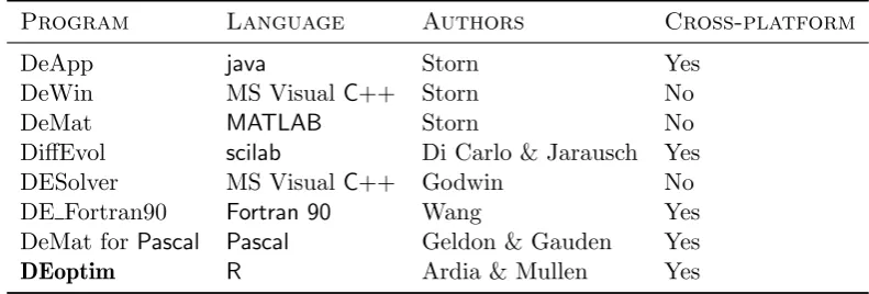
Program Language Authors Cross-platform
DeApp java Storn Yes
DeWin MS VisualC++ Storn No
DeMat MATLAB Storn No
DiffEvol scilab Di Carlo & Jarausch Yes
DESolver MS VisualC++ Godwin No
DE Fortran90 Fortran 90 Wang Yes
DeMat forPascal Pascal Geldon & Gauden Yes
[image:3.595.102.498.109.243.2]DEoptim R Ardia & Mullen Yes
Table 1: Implementations of Differential Evolution for general purpose optimization.
Many implementations of DE are currently available. A web-based list of DE programs for
general purpose optimization is maintained by Rainer Storn athttp://www.icsi.berkeley.
edu/~storn/code.html. A selection of programs from this list for which the source code
is readily available are summarized in Table 1. Commercial software such as Mathematica,
MATLAB’s GA toolbox, and a variety of special-purpose programs for optical and X-ray
physics also implement DE1.
The DEoptim implementation of DE was motivated by our desire to extend the set of
al-gorithms available for global optimization in the R language and environment for
statisti-cal computing (R Development Core Team 2009). R enables rapid prototyping of objective
functions, access to a wide array of tools for statistical modeling, and ability to generate
customized plots of results with ease (which in many situations makes use of R
prefer-able over the use of programs in languages like java, MS Visual C++, Fortran 90 or
Pas-cal). Furthermore, R is released in open-source form under the terms of the GNU General
Public License, meaning that packages implemented for it do not require the purchase of
commercial software. R also has a large and growing user base interested in optimization.
DEoptim has been published on the Comprehensive R Archive Network and is available at
http://cran.r-project.org/web/packages/DEoptim/. Since becoming publicly available
it has been used by a variety of authors, e.g., B¨orner, Higgins, Kantelhardt, and Scheiter
(2007), Higgins, Kantelhardt, Scheiter, and Boerner (2007), Cao, Vilar, and Devia (2009),
Opsina Arango (2009), and Ardia, Boudt, Carl, Mullen, and Peterson to solve optimization problems arising in diverse domains.
In the remainder of this manuscript we elaborate onDEoptim’s implementation and use. In
Section1.1, the package is introduced via a simple example. Section2describes the underlying
algorithm. Section3 describes theRimplementation and serves as a user manual. DEoptim
is then illustrated via two cases studies, involving fitting a Parratt recursion model for
X-ray reflectometry data (in Section 4) and a Markov-Switching Generalized Autoregressive
Conditional Heteroscedasticity(MSGARCH) model for log-returns of the Swiss Market Index
(in Section 5).
1Certain commercial equipment, instruments, or materials are identified in this paper to foster
x
1x
2−4
−2
0
2
4
−4 −2
0
2
4
●
[image:4.595.194.414.132.308.2]0
10
20
30
40
50
60
70
80
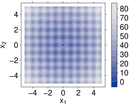
Figure 1: A contour plot of the two-dimensional Rastrigin functionf(x). The global minimum
f(x) = 0 is at (0,0) and is marked with an open white circle.
1.1. An introductory example
Minimization of the Rastrigin function inx∈ ℜD
f(x) =
D
X
j=1
x2j −10 cos (2πxj) + 10
forD= 2 is a common test for global optimization algorithms.
This function is possible to represent inRas
R> rastrigin <- function(x) 10 * length(x) + sum(x^2 - 10 * cos(2 * + pi * x))
As shown in Figure 1, for D = 2 the function has a global minimum f(x) = 0 at the point
(0,0).
In order to minimize this function using DEoptim, the R interpreter is invoked, and the
package is loaded with the command
R> library("DEoptim")
DEoptim package
Differential Evolution algorithm in R Authors: David Ardia and Katharine Mullen
The DEoptimfunction of the packageDEoptim searches for minima of the objective function between lower and upper bounds on each parameter to be optimized. Therefore in the call to
DEoptimwe specify vectors that comprise the lower and upper bounds; these vectors are the
R> est.ras <- DEoptim(rastrigin, lower = c(-5, -5), upper = c(5, + 5), control = list(storepopfrom = 1, trace = FALSE))
Note that the vector of parameters to be optimized must be the first argument of the objective
functionfn passed to DEoptim. The above call specifies the objective function to minimize,
rastrigin, the lower and upper bounds on the the parameters, and, via the control ar-gument, that we want to store intermediate populations from the first generation onwards (storepopfrom = 1), and do not want to print out progress information each generation (trace = FALSE). Storing intermediate populations allows us to examine the progress of the
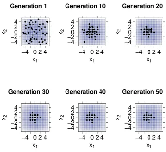
optimization in detail. Upon initialization, the population is comprised of 50 vectors x of
length two (50 being the default value ofNP), withxi a random value drawn from the uniform
distribution over the values defined by the associated lower and upper bound. The operations
of crossover, mutation, and selection explained in Section 2transform the population so that
the members of successive generations are more likely to represent the global minimum of the objective function. The members of the population generated by the above call are plotted at
the end of different generations in Figure2. DEoptim consistently finds the minimum of the
function within 200 generations using the default settings. We have observed that DEoptim
solves the Rastrigin problem more efficiently than the simulated annealing method found in
the Rfunctionoptim.
We note that as the dimensionality of the Rastrigen problem increases, DEoptim may not
be able to find the global minimum in the default number of generations. Heuristics to help ensure that the global minimum is found include re-running the problem with a larger
population size (value of NP), and increasing the maximum allowed number of generations.
1.2. When to apply DE
Differential Evolution does not require derivatives of the objective function. It is therefore useful in situations in which the objective function is stochastic, noisy, or difficult to differen-tiate. DE, however, may be inefficient on smooth functions, where derivative-based methods generally are most efficient.
For illustration, consider a generalized Rosenback function, possible to represent in Ras
R> genrose.f <- function(x) { + n <- length(x)
+ fval < 1 + sum(100 * (x[1:(n 1)]^2 x[2:n])^2 + (x[2:n]
-+ 1)^2)
+ return(fval) + }
This function has a global minimum at 1, which DEoptimfinds forn= 10 with a call like:
R> n <- 10
R> ans <- DEoptim(fn = genrose.f, lower = rep(-5, n), upper = rep(5, + n), control = list(NP = 100, itermax = 4000, trace = FALSE))
However, the minimum can be determined with far fewer function evalutations with a
Generation 10
x
1x
2−4
−2
0
2
4
−4 0 2 4
● ● ● ● ● ● ● ● ● ● ● ● ● ● ● ● ● ● ● ● ● ● ● ● ● ●● ● ● ● ● ● ● ● ● ● ● ● ● ● ● ● ● ● ●● ● ● ● ● ●
Generation 20
x
1x
2−4
−2
0
2
4
−4 0 2 4
● ● ● ● ● ● ● ● ● ● ● ● ● ● ● ● ● ● ● ● ● ● ● ● ● ● ● ● ● ● ● ● ● ● ● ● ● ● ●● ● ● ● ● ● ● ● ● ● ● ●
Generation 30
x
1x
2−4
−2
0
2
4
−4 0 2 4
● ● ● ● ● ● ● ● ● ● ● ● ● ● ● ● ● ● ● ● ● ● ● ● ● ● ● ● ● ● ● ● ● ● ● ● ● ● ● ● ● ● ●● ● ● ● ● ● ● ●
Generation 40
x
1x
2−4
−2
0
2
4
−4 0 2 4
● ● ● ● ● ● ● ● ● ● ● ● ● ● ● ● ● ● ● ● ● ● ● ● ● ● ●●● ● ● ● ● ● ●● ● ● ● ● ● ● ●● ● ● ● ● ● ● ●
Generation 50
x
1x
2−4
−2
0
2
4
−4 0 2 4
● ● ● ● ● ● ● ● ● ● ● ● ● ●● ● ● ● ● ● ● ● ● ● ● ● ●● ● ● ● ● ● ● ● ● ● ● ● ● ● ● ●● ● ● ● ● ● ● ●
Generation 1
x
1x
2−4
−2
0
2
4
−4 0 2 4
[image:6.595.125.468.239.552.2]● ● ● ● ● ● ● ● ● ● ● ● ● ● ● ● ● ● ● ● ● ● ● ● ● ● ● ● ● ● ● ● ● ● ● ● ● ● ● ● ● ● ● ● ● ● ● ● ● ● ●
Figure 2: The population associated with various generations of a call toDEoptimas it searches
for the minimum of the Rastrigin function (marked with an open white circle). The minimum
R> ans1 <- optim(par = runif(10, -5, 5), fn = genrose.f, method = "BFGS", + control = list(maxit = 4000))
Note further that users interested in exact reproduction of results should set the seed of their
random number generator before callingDEoptim. DE is a randomized algorithm, and the
results may vary between runs.
2. The Differential Evolution algorithm
We sketch the classical DE algorithm here and refer interested readers to the work ofStorn
and Price(1997) and Priceet al. (2006) for further elaboration. The algorithm is an evolu-tionary technique which at each generation transforms a set of parameter vectors, termed the population, into another set of parameter vectors, the members of which are more likely to minimize the objective function. In order generate a new parameter vector, DE disturbs an old parameter vector with the scaled difference of two randomly selected parameter vectors.
The variableNP represents the number of parameter vectors in the population. At generation
0, NP guesses for the optimal value of the parameter vector are made, either using random
values between upper and lower bounds for each parameter or using values given by the user. Each generation involves creation of a new population from the current population
membersxi,g, whereg indexes generation,iindexes the vectors that make up the population,
and j indexes into a parameter vector. This is accomplished using differential mutation of
the population members. A trial mutant parameter vector vi,g is created by choosing three
members of the population, xr0,g,xr1,g andxr2,g, at random. Thenvi,g is generated as
vi,g =xr0,g+ F·(xr1,g−xr2,g) (1)
whereF is a positive scale factor. Effective values of F are typically less than 1.
After the first mutation operation, mutation is continued until either length(x) mutations
have been made or rand>CR, whereCR is a crossover probability CR ∈[0,1], and where
here and throughout rand is used to denote a random number from U(0,1). The crossover
probabilityCRcontrols the fraction of the parameter values that are copied from the mutant.
CRapproximates but does not exactly represent the probability that a parameter value will
be inherited from the mutant, since at least one mutation always occurs.
If an elementvj of the parameter vector is found to violate the bounds after mutation and
crossover, it is reset. In the implementation DEoptim, if vj > upperj, it is reset as vj =
upperj −rand·(upperj −lowerj), and if vj < lowerj, it is reset as vj = lowerj + rand·
(upperj −lowerj). This ensures that candidate population members found to violate the
bounds are set some random amount away from them, in such a way that the bounds are guaranteed to be satisfied. Then the objective function values associated with the children
v are determined. If a trial vector vi,g has equal or lower objective function value than the
vectorxi,g,vi,g replaces xi,g in the population; otherwise xi,g remains. The algorithm stops
after some set number of generations, or after the objective function value associated with the best member has been reduced below some set threshold.
Variations on this theme are possible, some of which are described in the following section.
Values of rand and CR that have been found to be most effective for a variety of problems
are described inPriceet al.(2006) (Section 2). Reasonable default values for many problems
3. Implementation
DEoptimwas first published on the Comprehensive R Archive Network (CRAN) in 2005 by
David Ardia. Early versions were written in pureR. Since version 2.0-0 (published to CRAN
in 2009 by Katharine Mullen) the package has relied on an interface to aC implementation
of DE, which is significantly faster on most problems as compared to the implementation in
pureR. Since version 2.0-3 theCimplementation dynamically allocates the memory required
to store the population, removing limitations on the number of members in the population and length of the parameter vectors that may be optimized.
The implementation is used by calling theRfunctionDEoptim, the arguments of which are:
• fn: The objective function to be minimized. This function should have as its first
argument the vector of real-valued parameters to optimize, and return a scalar real result.
• lower,upper: Vectors specifying scalar real lower and upper bounds on each parameter
to be optimized, so that theith element oflowerandupperapplies to theith parameter.
The implementation searches between lower andupper for the global optimum offn.
• control: A list of control parameters, discussed below.
• ...: allows the user to pass additional arguments to the function fn.
Thecontrol argument is a list, the following elements of which are currently interpreted:
• VTR: The value to reach. Specify the global minimum offnif it is known, or if you wish
to cease optimization after having reached a certain value. The default value is-Inf.
• strategy: This defines the Differential Evolution strategy used in the optimization
procedure, described below in the terms used by Priceet al. (2006):
– 1: DE / rand / 1 / bin (classical strategy). This strategy is the classical approach
described in Section 2.
– 2: DE / local-to-best / 1 / bin. In place of the classical DE mutation given in (1),
the expression
vi,g = oldi,g+ (bestg−oldi,g) +xr0,g+ F·(xr1,g−xr2,g)
is used, where oldi,g and bestg are theith member and best member, respectively,
of the previous population. This strategy is currently used by default.
– 3: DE / best / 1 / bin with jitter. In place of the classical DE mutation given in
(1), the expression
vi,g= bestg+ jitter + F·(xr1,g−xr2,g)
is used, where jitter is defined as 0.0001·rand +F.
– 4: DE / rand / 1 / bin with per vector dither. In place of the classical DE mutation
given in (1), the expression
vi,g=xr0,g+ dither·(xr1,g−xr2,g)
– 5: DE / rand / 1 / bin with per generation dither. The strategy described for4is
used, but dither is only determined once per-generation.
– any value not above: variation to DE / rand / 1 / bin: either-or algorithm. In the
case that rand<0.5, the classical strategy described for1is used. Otherwise, the
expression
vi,g =xr0,g+ 0.5·(F+ 1.0)·(xr1,g+xr2,g−2·xr0,g)
is used.
• bs: If FALSE then every mutant will be tested against a member in the previous
gen-eration, and the best value will survive into the next generation. This is the standard
trial vs. target selection described in Section 2. If TRUE then the old generation and
NP mutants will be sorted by their associated objective function values, and the bestNP
vectors will proceed into the next generation (this is best-of-parent-and-child selection).
The default value is FALSE.
• NP: Number of population members. The default value is50.
• itermax: The maximum iteration (population generation) allowed. The default value
is 200.
• CR: Crossover probability from interval [0,1]. The default value is0.9.
• F: Stepsize from interval [0,2]. The default value is0.8.
• trace: Logical value indicating whether printing of progress occurs at each iteration.
The default value is TRUE.
• initialpop: An initial population used as a starting population in the optimization
procedure, specified as a matrix in which each row represents a population member.
May be useful to speed up convergence. Defaults toNULL, so that the initial population
is generated randomly within the lower and upper boundaries.
• storepopfrom: From which generation should the following intermediate populations
be stored in memory. Default toitermax+1, i.e., no intermediate population is stored.
• storepopfreq: The frequency with which populations are stored. The default value is
1, i.e. every intermediate population is stored.
• checkWinner: Logical value indicating whether to re-evaluate the objective function
using the winning parameter vector if this vector remains the same between gener-ations. This may be useful for the optimization of a noisy objective function. If
checkWinner=TRUE and avWinner=FALSE then the value associated with re-evaluation
of the objective function is used in the next generation. Default to FALSE.
• avWinner: Logical value. If checkWinner=TRUE and avWinner=TRUE then the
objec-tive function value associated with the winning member represents the average of all evaluations of the objective function over the course of the ‘winning streak’ of the best population member. This option may be useful for optimization of noisy objective
0.01 0.02 0.03 0.04 0.05 0.06 0.07
1e+02
1e+06
θ (radians)
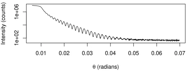
[image:10.595.127.458.150.278.2]Intensity (counts)
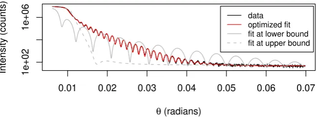
Figure 3: XRR measurements of Pt layers on SiO2 substrate.
The default value of controlis the return value ofDEoptim.control(), which is a list with
the above elements and specified default values.
The return value of the DEoptim function is a member of the S3 class DEoptim. Members
of this class have a plot method that accepts the argument plot.type. When retVal is
an object returned by DEoptim, calling plot(retVal, plot.type = "bestmemit") results
in a plot of the parameter values that represent the lowest value of the objective function
each generation. Calling plot(retVal, plot.type = "bestvalit") plots the best value of
the objective function each generation. Calling plot(retVal, plot.type = "storepop")
results in a plot of stored populations (which are only available if these have been saved by
setting the control argument of DEoptim appropriately). A summary method for objects
of S3 class DEoptim also exists, and returns the best parameter vector, the best value of the
objective function, the number of generations optimization ran, and the number of times the objective function was evaluated.
A note on recommended settings: we have set the default values to the methods recommended by Price et al. (2006) as starting points. We use strategy=2 by default; the user should
consider trying as alternativesstrategy=6andstrategy=1, though the best method will be
highly problem-dependent. Generally, the user should set the lower and upper bounds to to exploit the full allowable numerical range, i.e., if a parameter is allowed to exhibit values in the range [-1, 1] it is typically a good idea to pick the initial values from this range instead of
unnecessarily restricting diversity. Increasing the value forNP will mean greater likelihood of
finding the minimum, but run-time will be longer.
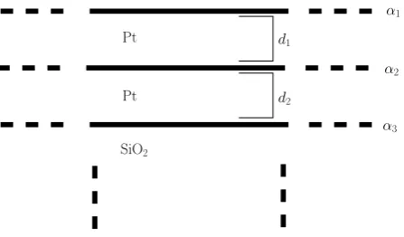
4. Application I: X-ray reflectometry
X-ray reflectometry (XRR) is a measurement method that uses the interference of X-rays (i.e., photons with a wavelength in the approximate range of 0.01 nm–10 nm) caused by changes in a material’s electron density to characterize thin films or other layered structures at the nanometer to micrometer scale. The data collected consists of pairs of incident/scattered
Pt
Pt
d1
d2
SiO2
α1
α2
[image:11.595.198.422.164.295.2]α3
Figure 4: Schematic description of two layers of Pt on a substrate of SiO2. A Parratt recursion
model representing this structure will be fit to the XRR measurements, with free parameters
including the thickness of the Pt layers (d1 andd1), and terms (ρ1,ρ2, andρ3) describing the
roughness of the interfaces between layers.
Information regarding the density and thickness of each layer, and on the roughness of the interface between layers and at the surface of the material is extracted by fitting a parametric model to the measurements.
In the supplementary information we provide the full description of a model function used by DEoptimto obtain physically realistic parameter estimates from the data shown in Figure
3. This model is based on the Parratt recursion (Parratt 1954), which, as Als-Nielsen and
McMorrow(2001) describe in detail, is often used to model each of the layers in multilayered materials. For the data here, the Parratt recursion is used to describe reflection and transmis-sion of X-rays from two thin layers of Pt (with each layer having a possibly distinct thickness,
density, and roughness at the interface) atop an infinitely thick layer of SiO2. Figure 4 is a
schematic description of the model for this multilayered material.
The free parameters of the applied Parratt recursion model are the thicknessesd1 and d2 of
each Pt layer, the density σ1 and σ2 of each Pt layer, terms ρ1,ρ2 and ρ3 descriptive of the
roughness of the interfaces between layers and at the surface, a parameterbdescribing a linear
background, and a multiplicative scaling parameterm. The model function can be understood
qualitatively by considering the the case of a single layer on a substrate. In this case, the position of the abrupt drop-off in scattered intensity after the initial plateau is determined by the density of the layer. The period of the subsequent oscillation fringes is set by the thickness of the layer, whereas the decay of the oscillations is a function of the roughness of the layer. Because the amplitudes of reflected and transmitted waves interfere, this qualitative view cannot be extended to multilayered systems and model fitting is a necessity.
The objective function R to minimize is formulated as the sum of the squared differences
0.01 0.02 0.03 0.04 0.05 0.06 0.07
1e+02
1e+06
θ (radians)
Intensity (counts)
[image:12.595.130.455.153.274.2]data optimized fit fit at lower bound fit at upper bound
Figure 5: XRR measurements (black) of Pt layers on SiO2 substrate with model fit (red).
For comparison, the model has also been evaluated at the lower and upper bounds on the
parameters used in the call to DEoptim(solid and dashed grey, respectively).
optimization algorithm such as DE. Treatment of global optimization problems such as these have been successfully addressed for many years in the XRR community using DE as, e.g.,
Wormington, Panaccione, Matney, and Bowen (1999), Taylor, Wall, Loxley, Wormington, and Lafford(2001), andBowen and Tanner (2006) describe. Special purpose programs, e.g.,
theGenX program developed byBj¨orck and Andersson (2007) and theMOTOFITprogram
developed byNelson (2006), have been implemented for XRR model fitting problems of this
sort.
The XRR measurements shown in Figure3are included inDEoptimas the datasetxrrData,
with the vector of data to be fit represented by the vector counts. We have encoded the
objective functionR as the functionrss. Using knowledge of the physical system underlying
the measurements in order to set plausible lower and upper bounds on the parameters to
optimize, and to set fixed values forbeta,wavelength, and delta, the objective function is
minimized with the call
R> parrattFit <- DEoptim(lower = c(d_1 = 5.5e-10, d_2 = 1.5e-08,
+ rho_1 = 2.1e-10, rho_2 = 5.0e-12, rho_3 = 2.2e-10, + alpha_1 = 10, alpha_2 = 10, b = 40, m = .90e7), + upper = c(d_1 = 5.5e-09, d_2 = 1.5e-07,
+ rho_1 = 2.1e-09, rho_2 = 5.0e-11, rho_3 = 2.2e-09, + alpha_1 = 21.46, alpha_2 = 21.46, b = 55, m = 1.1e7), + fn = rss, theta_r = theta_r, delta = delta,
+ beta = beta, wavelength = wavelength, data = counts, + control = list(itermax = 1500, NP = 90))
Table 2 gives parameter estimates arrived at via the above call, along with the associated
lower and upper bounds. The resulting fit of the model to the data is shown in Figure5. The
upper bound for the density of the Pt layers was set at 21.46 g·cm−3, the density of Pt in
bulk. The estimates for the densities (19.6 g·cm−3 and 20.9 g·cm−3) are slightly lower than
d1 d2 ρ1 ρ2 ρ3 σ1 σ2 b m
/ nm / g·cm−3 / counts
lower 0.55 15.0 0.21 0.005 0.22 10.0 10.0 40.0 0.90e7
upper 5.50 150.0 2.10 0.050 2.20 22.0 22.0 55.0 1.20e7
bestmem 1.69 45.6 0.62 0.0053 0.69 20.0 21.0 48.0 1.1e7
Table 2: Parameter estimates (bestmem) and lower and upper bounds associated with the
call to DEoptim that results in the fit of Parratt recursion model to XRR data shown in
Figure 5. Parameters d1 and d2 represent the thickness of the Pt layers, parameters ρ1,
ρ2, ρ3 describe the roughness of the interfaces between layers, and parameters σ1 and σ2
represent the density of the Pt layers. Parameterbrepresents an additive background term,
and parameter m represents a multiplicative scaling factor for the intensity. Estimates are
reported to two significant figures, except fort1 and t2, which are reported to three.
first principles, though the evaluation of the ability of the model to describe the material underlying the XRR measurements is beyond the scope of this paper. As shown in Figure
5, the model fit captures the qualitative features of the dataset well. The robustness of the
estimates has been validated via initialization of DE using a variety of starting populations;
the estimates presented in Table2reliably represent the best results obtained.
The functionrssencoding the objective function can easily be customized to the dataset at
hand, allowing, for instance, inclusion of more or fewer free parameters. Note that in this
example, the population size, NP, was set to 90 since in practice it has been observed that
convergence to the global optimum is facilitated if NP is at least ten times the number of
parameters being optimized (Price et al.2006). Determination of whether the best member
returned byDEoptim with this call represents a unique global minimum is beyond the scope
of this paper, but would be interesting to check for the purpose of developing a physical interpretation of the model fit.
5. Application II: Log-returns of the Swiss Market Index
Volatility plays a central role in empirical finance and financial risk management. Research on changing volatility (i.e., conditional variance) using time series models has been active since the creation of the original ARCH (AutoRegressive Conditional Heteroscedasticity) and GARCH (Generalized ARCH) models. Since then, GARCH type models grew rapidly into a rich family of empirical models for volatility forecasting during the last twenty years. They are now widespread and essential tools in financial econometrics.
In the GARCH(p, q) specification introduced by Bollerslev (1986), the conditional variance
at time t of the log-return yt (of a financial asset or a financial index), denoted by σt2, is
postulated to be a linear function of the squares of pastq log-returns and pastp conditional
variances. More precisely:
σt2 =. α0+
q
X
i=1
αiyt2−i+ p
X
j=1
where the parameters α0 > 0, αi ≥ 0 (i = 1, . . . , q) and βj ≥ 0 (j = 1, . . . , p) in order to
ensure a positive conditional variance. In most empirical applications it turns out that the
simple specification p =q = 1 is able to reproduce the volatility dynamics of financial data.
This has led the GARCH(1,1) model to become the workhorse model by both academics and
practitioners.
Numerous extensions and refinements of the GARCH(1,1) model have been proposed to mimic additional stylized facts observed in financial markets, such as nonlinearity, asymmetry, and
long memory properties in the volatility process; seeBollerslev, Chou, and Kroner(1992) and
Bollerslev, Engle, and Nelson(1994) for a review. Among them, the class of Markov-switching GARCH (MSGARCH) has gained particular attention in recent years. In these models, the
parameters of the scedastic function (2) can change over time according to a latent (i.e.,
unobservable) variable taking values in the discrete space {1, . . . , K} where K is an integer
defining the number of regimes or states. The interesting feature of these models lies in the fact that they provide an explanation of the high persistence in volatility, i.e., nearly unit root
process for the conditional variance, observed with single-regime GARCH models (Lamoureux
and Lastrapes 1990). Furthermore, these models are apt to react quickly to changes in the volatility level (unconditional volatility) which leads to significant improvements in volatility
forecasts as shown by Dueker (1997) or Klaassen (2002) for instance. These features make
the models attractive for various applications in financial modeling, such as risk management. While MSGARCH models are attractive for the description of a variety of phenomena, we face practical difficulties when attempting to fit their parameters to data. The maximization of the likelihood function is a constrained optimization problem since some (or all) of the model parameters must be positive to ensure a positive conditional variance. It is also common to require that the covariance stationarity condition holds; this leads to additional non-linear inequality constraints which render the optimization procedure cumbersome. Optimization results are often sensitive to the choice of starting values. Finally, convergence is hard to achieve if the true parameter values are close to the boundary of the parameter space and if the underlying process is nearly non-stationary. For these reasons, a robust optimizer is required. DE offers an adequate approach to finding the maximum likelihood parameter estimates in this framework.
In order to illustrate the robustness of DEoptim compared to traditional estimation
tech-niques, we consider a two-state asymmetric MSGARCH model investigated in Ardia (2008,
chapter 7). The author illustrated the poor performance of traditional local optimizers when estimating such sophisticated models. Only computationally demanding Markov chain Monte Carlo techniques were able to provide meaningful results.
A two-state Markov-switching asymmetric GARCH(1,1) model with Student-t innovations
for the log-returns{yt} may be written as
yt=εt
q
ν−2
ν σs2t,t t= 1, . . . , T ,
εt
i.i.d.
∼ S(0,1, ν),
σi,t2 =.
(
ω1+ α+11{yt−1≥0}+α −
11{yt−1<0}
y2
t−1+β1σ12,t−1 when st= 1
ω2+ α+21{yt−1≥0}+α −
21{yt−1<0}
yt2−1+β2σ22,t−1 when st= 2,
(3)
parameterν ensures that the conditional variance σ2
i,t remains finite; the restrictions on the
GARCH parameters ωi, α+i , α−i and βi guarantee its positivity. t is the time index and T
denotes the total number of observations. 1{·} denotes the indicator function which is equal
to one if the constraint holds and zero otherwise. The sequence {st} is assumed to be a
stationary, irreducible Markov process with discrete state space{1,2}and transition matrix
P = [. pij] where pij =. P(st+1 = j|st =i) is the transition probability of moving from state
i to state j (i, j ∈ {1,2}). Finally, S(0,1, ν) denotes the standard Student-t density with
ν degrees of freedom and p
(ν−2)/ν is a scaling factor which ensures that the conditional
variance ofyt isσ2st,t.
Model specification (3) allows reproduction of the so-called volatility clustering observed in
financial returns, i.e., the fact that large changes tend to be followed by large changes (of either sign) and small changes tend to be followed by small changes. Moreover, it allows for sudden
changes in the unconditional variance of the process; in the ith regime, the unconditional
variance is
¯
σ2i =. ωi
1−(α+i +α−i )/2−βi
, (4)
provided that (αi++α−i )/2 +βi <1 (i.e., the process is covariance stationary); see Bollerslev
(1986, page 310). Finally, it allows determination of whether or not an asymmetric response is
present (i.e.,α−i > α+i for at least onei) and is different between the regimes (i.e.,αi−6=α−i′).
This asymmetric response, referred to as the leverage effect in the financial literature, reflects
the fact that the volatility tends to rise more in response to bad news (i.e.,yt−1 <0) than to
good news (i.e.,yt−1 ≥0).
In order to write the likelihood function corresponding to model (3), we define the vector of
log-returnsy= (. y1, . . . , yT)′ and we regroup the eleven model parameters into the vector
θ= (. ω1, ω2, α+1, α+2, α1−, α−2, β1, β2, p11, p22, ν)′.
The conditional density ofytin statest=igivenθand the information setIt−1 =. {yt−1, . . . , y1}
is
f(yt|st=i, θ, It−1) =
Γ ν+12
Γ ν2q
π(ν−2)σ2
i,t
"
1 + y
2
t
σi,t2 (ν−2)
#(ν+1)/2 ,
where Γ(·) denotes the Gamma function. This stems from the fact that in state i,yt follows
a Student-t distribution with mean zero, varianceσ2
i,t and degrees of freedomν.
By integrating out the state variablest, we can obtain the density ofytgivenθandIt−1only.
The (discrete) integration is obtained as follows:
f(yt|θ, It−1) = 2
X
i=1 2
X
j=1
whereηi,t−1 =. P(st−1 =i|θ, It−1) is thefiltered probability of state iat timet−1 and where
we recall that pij denotes the transition probability of moving from state i to state j. The
filtered probabilities{ηi,t;i= 1,2;t= 1, . . . , T}are obtained by an iterative algorithm similar
in spirit to a Kalman filter; we refer the reader to Hamilton (1989) and Hamilton (1994,
chapter 22) for details.
Finally, the log-likelihood function corresponding to model specification (3) is obtained from (5)
as follows:
L(θ|y)=.
T
X
t=2
lnf(yt|θ, It−1). (6)
The maximum likelihood estimator ˆθis obtained by maximizing (6) (or minimizing its negative
value).
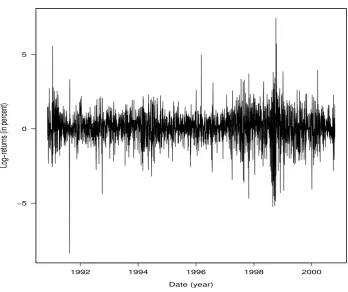
To illustrate the utility ofDEoptim, we fit the MSGARCH model (3) to daily log-returns of
the Swiss Market Index (SMI), displayed in Figure 6. The sample period is from November
12, 1990, to October 20, 2000, for a total of 2500 observations and the log-returns are
ex-pressed in percent. The data set was downloaded fromhttp://www.finance.yahoo.comand
is available whenDEoptimis loaded using the commanddata(SMI). Note that the two-regime
specification is used for illustrative purposes only; checking for possible model misspecification is beyond the scope of the present paper.
In addition to the positivity constraints on the model parameters, we require covariance stationarity to hold in the two regimes, i.e., (α+i +α−i )/2 +βi <1 fori= 1,2 and that the
unconditional variance (4) in state 1 is smaller than in state 2, i.e., ¯σ12 <σ¯22. We also require
the transition probabilities p11 and p22 of the state variable to lie within the [0,1] interval.
The constraints on the domain are set using the arguments lower and upper of DEoptim,
while the covariance stationarity and unconditional variance constraints are tested within the
objective function which then returns a very large value (in our case1e10) if not satisfied. In
the DE optimization, we set the control parameters of DEoptim toitermax = 500 and NP
= 110. Note that the objective function (6) is implemented inCto speed up the optimization
procedure. We refer the reader to the Appendix for details on the Rimplementation.
For comparison, the objective function (6) is also optimized using various unconstrained
and constrained optimization routines available in R. More specifically, we use the function
optim with methods"Nelder-Mead" (unconstrained optimization), "BFGS" (unconstrained),
"CG" (unconstrained), "SANN" (unconstrained), "L-BFGS-B" (box constrained), the function
nlminb (box constrained). More details on the underlying algorithms for these methods can
be found in the optim and nlminb manuals. We also consider optimization routines which
handle more complicated constraints such as constrOptim, constrOptim.nl of the package
alabama (Varadhan 2010) and solnp of the package Rsolnp (Ghalanos and Theussl 2010). The former relies on an adaptive barrier algorithm and handles linear inequality constraints. The two latter belong to the class of indirect solvers and implement the augmented Lagrange multiplier methods, in which linear and non-linear equality and inequality constraints are
allowed; seeYe(1987) for details. For all methods we use ten times the default values of the
control parameters related to the maximum number of iterations and function evaluations. For optim with method "SANN" we set itermax = 1e5. For unconstrained methods, the
−5 0 5
Date (year)
Log−retur
ns (in percent)
[image:17.595.119.468.126.418.2]1992 1994 1996 1998 2000
Figure 6: SMI daily log-returns.
satisfied, as forDEoptim. For functions which handled inequality constraints, we implement
the constraints explicitly in the inputs of the functions; see the Appendix for an example with
solnp.
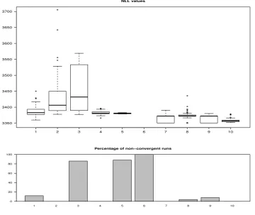
We run the estimation 50 times for all optimization routines (including DEoptim) and use
random starting values in the feasible parameter set when needed (using the same random starting values for the various methods). Boxplots of the negative log-likelihood value (NLL)
at optimum for convergent estimations is displayed in the upper part of Figure 7. The
lower part reports the percentage of non-convergent optimizations (defined asNaN output or
non-convergent flag, usuallyconvergence > 0). We notice that the unconstrained and box
constrained methods 1-6 perform poorly compared to the optimizers which can handle more
complicated constraints. In particular, we note that nlminb does not converge over the 50
runs. Overall, the methodssolnpandconstrOptimare the best performers in terms of lowest
NLL values reached over the 50 runs. However, we notice that for both the convergence is not
achieved in about 20% of the time. DEoptimcompares favorably with the two best competitors
and is more stable over the runs. It does not however reach the lowest value obtained bysolnp
after 500 iterations.
Figure 8 displays the boxplots of the NLL values obtained over the 50 runs of DEoptimwith
control parameter itermax = 500 on the left-hand side and itermax = 1000 on the
right-hand side. The horizontal red lines reports the lowest values obtained by solnp. We notice
toward the global optimum.
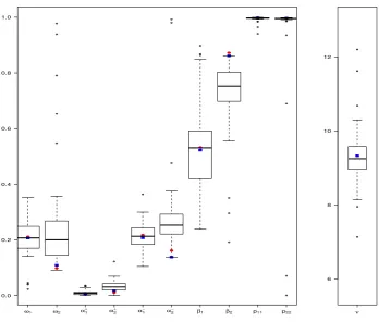
Figure9displays the boxplots of the parameter values obtained with the 50 runs of DEoptim
together with the parameter values corresponding to its best run (in blue squares), i.e., the run leading to the minimum NLL, and the parameter values corresponding to the best run of
solnp(in red dots). The parameters at theglobal optimum (NLL = 3350.6979) obtained by
solnpandDEoptim (after a longer run withitermax = 2500) are ˆω1= 0.2062, ˆω2 = 0.0930,
ˆ
α+1 = 0.0000, ˆα+2 = 0.0043, ˆα−1 = 0.2123, ˆα−2 = 0.1566, ˆβ1 = 0.5295, ˆβ2 = 0.8717, ˆp11 =
0.9981, ˆp22 = 0.9969 and ˆν = 9.2480. The parameter estimates clearly indicate two different
regimes for the conditional variance process. More precisely, the values of ˆωi and ˆβi are far
apart between the regimes. We note the presence of leverage effect in both regimes (i.e., ˆ
α+i <αˆ−i fori= 1,2), with similar levels. The estimated transition probabilities ˆp11 and ˆp22
very close to one indicate infrequent mixing between states. Finally, the estimated degrees of freedom parameter suggests heavy tails for the conditional distribution of the log-returns.
Finally, Figure10displays the estimated filtered probabilities of the second state (high
uncon-ditional volatility state),{P(st= 2|θ, Iˆ t);t= 1, . . . , T}, implied by the best model parameters
of solnp (in red solid line) together with the log-returns (in small circles). In addition, we
report in dashed blue lines, the 50% area of the paths obtained over the 50 runs ofDEoptim.
The parameters obtained withDEoptimandsolnplead to a clear separation of regimes in the
filtering probabilities. The beginning of year 1991 is associated with the high unconditional volatility state. Then, from the second half of 1991 to 1997, the returns are clearly associated with the low unconditional volatility regime, with the exception of 1994. From 1997 to 2000, the model remains in the high unconditional volatility regime with a transition during the second semester 2000 to the low unconditional volatility state.
6. Summary and conclusions
Differential Evolution is a heuristic evolutionary method for global optimization that is effec-tive on many problems of interest in science and technology. By implementing the package
DEoptim we have made this algorithm possible to easily apply in the Rlanguage and
envi-ronment. As Section 3 details, we have also made available many variations on the classical
DE strategy. These variations as well as the classical strategy are due to Price, Storn and
Lampinen, and we have referred the interested reader to their textbook (Priceet al.2006) on
DE for details.
We have described herein the use of the package for fitting the Parratt recursion models for X-ray reflectometry and an MSGARCH model for the log-returns of the Swiss Market Index.
These case studies showcase the power of the DE algorithm underlying DEoptim. We hope
that readers will find the package to be a valuable tool for optimization. If you use R or
DEoptim, please cite the software in publications.
Current work in extension of the package includes the addition of a framework for adaptive
Differential Evolution (Zhang and Sanderson 2009). Future work will also be directed at
parallization of the implementation. The DEoptim project hosted on R-forge (https://
Computational details
The results in this paper were obtained usingR2.10.0 (RDevelopment Core Team 2009) with
the packagesDEoptimversion 2.0-4 (Ardia and Mullen 2009). Computations were performed
on a Genuine Intel dual core CPU T2400 1.83Ghz processor and on a quad core Intel Xeon Processor E5410.
DEoptimrelies on repeated evaluation of the objective function in order to move the
popula-tion toward a global minimum. Users interested in makingDEoptim run as fast as possible
should ensure that evaluation of the objective function is as efficient as possible. Using pure
Rcode, this may often be accomplished using vectorization. Writing parts of the objective
function in a lower-level language likeC orFortran may also increase speed.
Acknowledgements
Many DEoptimusers have sent us comments that helped improve the package. We would like to thank in particular Hans Werner Borchers, Eugene Demidenko, Tarmo Leinonen, Soren Macbeth, Doroth´ee Pages, Brian Peterson, Enrico Schumann, and Joshua Ulrich. We would also like to thank Juan David Ospina Arango, who inspired us to present the Rastrigin function as an example.
We thank the two reviewers of the paper for insightful suggestions.
Finally, we would like to thank Rainer Storn for his advocacy of DE and making his code
publicly available, which was a great help to us in the implementation of DEoptim.
Disclaimer
The views expressed in this chapter are the sole responsibility of the authors and do not necessarily reflect those of NIST and aeris CAPITAL AG.
Certain commercial equipment, instruments, or materials are identified in this paper to foster understanding. Such identification does not imply recommendation or endorsement by the National Institute of Standards and Technology, nor does it imply that the materials or equipment identified are necessarily the best available for the purpose.
References
Als-Nielsen J, McMorrow D (2001). Elements of Modern X-ray Physics. Wiley.
Ardia D (2008). Financial Risk Management with Bayesian Estimation of GARCH
Models: Theory and Applications, volume 612 of Lecture Notes in Economics and Mathematical Systems. Springer-Verlag, Berlin, Germany. ISBN 978-3-540-78656-6. doi:10.1007/978-3-540-78657-3. URL http://www.springer.com/economics/ econometrics/book/978-3-540-78656-6.
Ardia D, Mullen K (2009). DEoptim: Differential Evolution Optimization in R. R package
version 2.00-04, URLhttp://CRAN.R-project.org/package=DEoptim.
Bj¨orck M, Andersson G (2007). “GenX: An Extensible X-ray Reflectivity Refinement Program
Utilizing Differential Evolution.”Journal of Applied Crystallography,40(6), 1174–1178.
Bollerslev T (1986). “Generalized Autoregressive Conditional Heteroskedasticity.” Journal of
Econometrics,31(3), 307–327. doi:10.1016/0304-4076(86)90063-1.
Bollerslev T, Chou RY, Kroner K (1992). “ARCH Modeling in Finance: A Review
of the Theory and Empirical Evidence.” Journal of Econometrics, 52(1–2), 5–59.
doi:10.1016/0304-4076(92)90064-X.
Bollerslev T, Engle RF, Nelson DB (1994). “ARCH Models.” In Handbook of Econometrics,
chapter 49, pp. 2959–3038. North Holland.
B¨orner J, Higgins SI, Kantelhardt J, Scheiter S (2007). “Rainfall or Price
Variabil-ity: What Determines Rangeland Management Decisions? A Simulation-Optimization
Approach to South African Savanas.” Agricultural Economics, 37(2–3), 189–200.
doi:10.1111/j.1574-0862.2007.00265.x.
Bowen DK, Tanner BK (2006). X-Ray Metrology in Semiconductor Manufacturing. CRC.
Byrd RH, Lu P, Nocedal J, Zhu CY (1995). “A Limited Memory Algorithm for Bound
Constrained Optimization.”SIAM Journal on Scientific Computing,16(6), 1190–1208.
Cao R, Vilar JM, Devia A (2009). “Modelling Consumer Credit Risk via Survival Analysis.”
Statistics & Operations Research Transactions,33(1), 3–30.
Dueker MJ (1997). “Markov Switching in GARCH Processes and Mean-Reverting
Stock-Market Volatility.” Journal of Business & Economic Statistics,15(1), 26–34.
Ghalanos A, Theussl S (2010). Rsolnp: General Non-linear Optimization Using Augmented
Lagrange Multiplier Method. R package version 1.0-4.
Hamilton JD (1989). “A New Approach to the Economic Analysis of Nonstationary Time
Series and the Business Cycle.”Econometrica,57(2), 357–384.
Hamilton JD (1994). Time Series Analysis. First edition. Princeton University Press,
Prince-ton, USA. ISBN 0691042896.
Higgins SI, Kantelhardt J, Scheiter S, Boerner J (2007). “Sustainable Management of
Extensively Managed Savanna Rangelands.” Ecological Economics, 62(1), 102–114.
doi:10.1016/j.ecolecon.2006.05.019.
Holland JH (1975). Adaptation in Natural Artificial Systems. University of Michigan Press,
Ann Arbor.
Klaassen F (2002). “Improving GARCH Volatility Forecasts with Regime-Switching GARCH.”
Empirical Economics,27(2), 363–394. doi:10.1007/s001810100100.
Lamoureux CG, Lastrapes WD (1990). “Persistence in Variance, Structural Change, and the
Mitchell M (1998). An Introduction to Genetic Algorithms. The MIT Press.
Nelson A (2006). “Co-refinement of multiple-contrast neutron/X-ray
reflectiv-ity data using MOTOFIT.” Journal of Applied Crystallography, 39(2), 273–
276. doi:10.1107/S0021889806005073. URL http://dx.doi.org/10.1107/ S0021889806005073.
Opsina Arango JD (2009). Estimacion de un Modelo de Difusion con Saltos con
Distribu-cion de Error Generalizada Asimetrica usando Algorithmos Evolutivos. Master’s thesis, Universidad Nacional de Colombia.
Parratt LG (1954). “Surface Studies of Solids by Total Reflection of X-Rays.”Physical Review,
95(2), 359–369.
Price KV, Storn RM, Lampinen JA (2006). Differential Evolution: A Practical Approach to
Global Optimization. Springer-Verlag, Berlin, Germany. ISBN 3540209506.
RDevelopment Core Team (2009).R: A Language and Environment for Statistical Computing.
RFoundation for Statistical Computing, Vienna, Austria. ISBN 3-900051-07-0, URLhttp:
//www.R-project.org.
Storn R, Price K (1997). “Differential Evolution – A Simple and Efficient Heuristic for Global
Optimization over Continuous Spaces.” Journal of Global Optimization, 11(4), 341–359.
ISSN 0925-5001.
Taylor M, Wall J, Loxley N, Wormington M, Lafford T (2001). “High resolution X-ray
Diffrac-tion Using a High Brilliance Source, with Rapid Data Analysis by Auto-fitting.”Materials
Science and Engineering B,80(1-3), 95 – 98. ISSN 0921-5107.
Varadhan R (2010). alabama: Constrained Nonlinear Optimization. R Package version
2010.7-1.
Wormington M, Panaccione C, Matney KM, Bowen DK (1999). “Characterization of
Struc-tures from X-ray Scattering Data Using Genetic Algorithms.”Philosophical Transactions of
the Royal Society of London. Series A: Mathematical, Physical and Engineering Sciences,
357(1761), 2827–2848. doi:10.1098/rsta.1999.0469.
Ye Y (1987).Interior Algorithms for Linear, Quadratic, and Linearly Constrained Non-Linear
Programming. Ph.D. thesis, Department of ESS, Stanford University.
Zhang J, Sanderson AC (2009). “JADE: adaptive Differential Evolution
with optional external archive.” Trans. Evol. Comp, 13(5), 945–958.
1 2 3 4 5 6 7 8 9 10 3350
3400 3450 3500 3550 3600 3650 3700
NLL values
1 2 3 4 5 6 7 8 9 10
0 20 40 60 80 100
[image:22.595.119.480.203.506.2]Percentage of non−convergent runs
Figure 7: Top: Boxplots of the 50 negative values of the log-likelihood function (NLL) at
opti-mum ˆθ obtained by the various optimizers. (1) functionoptimwith method"Nelder-Mead",
(2) method "BFGS", (3) method "CG", (4) method "L-BFGS-B", (5) method "SANN" with
control parameteritermax = 1e5, (6) functionnlminb, (7) functionconstrOptim, (8)
func-tion constrOptim.nl of the package alabama, (9) function solnp of the package Rsolnp,
(10) functionDEoptim with control parametersNP = 110 and itermax = 500. Starting
val-ues are generated randomly in the feasible parameter set. Lower boundaries were set to 0.0
(2.0 for ν) and upper boundaries to 1.0 (50 for ν). Bottom: Percentage of non-convergent
runs of the different optimization methods (eitherNaNoutput or convergence flag indicating
itermax = 500 itermax = 1000 3350
[image:23.595.152.443.248.531.2]3355 3360 3365 3370
Figure 8: Top: Boxplots of the 50 negative values of the log-likelihood function (NLL) at
optimum ˆθobtained byDEoptimwith control parametersNP = 110anditermax = 500(left)
ω1 ω2 α1+ α2+
α1− α2−
β1 β2 p11 p22
0.0 0.2 0.4 0.6 0.8 1.0
6 8 10 12
[image:24.595.126.475.254.550.2]ν
Figure 9: Boxplot of the parameters obtained over the 50 runs ofDEoptim, together with the
parameters of its best run (blue squares), i.e., the run leading to the lowest NLL, and the
0.0 0.2 0.4 0.6 0.8 1.0
Date (year)
Pr(
[image:25.595.117.468.254.546.2]st
= 2 |
θ
^ , I
t
)
1992 1994 1996 1998 2000
Figure 10: Estimated filtered probabilities of the second state,{P(st= 2|θ, Iˆ t);t= 1, . . . , T},
implied by the best model parameters obtained by solnp (in red) over the 50 runs. The
dashed blue lines delimit the 50% area of the paths obtained over the 50 runs ofDEoptim.
A. Implementation of the MSGARCH model
We described below the major steps for implementing and estimating in R the
Markov-switching asymmetric GARCH(1,1) model described in Section5.
First, we define the functionNLLwhich computes the negative value of the log-likelihood
func-tion (6). This function will be minimized in order to find the maximum likelihood estimator ˆθ.
The functionNLLhas input parameterstheta, a 11-dim vector containing the MSGARCH(1,1)
parameters, ythe (T ×1) vector of log-returns y = (. y1, . . . , yT)′ and checkConstraints, a
boolean indicating if the constraints should be checked within the function (which is TRUE
by default). The function outputs 1e10 when the constraints are not fulfilled. In the
imple-mentation below, two constraints must be fulfilled: i) the covariance-stationarity condition of the conditional variance is satisfied in the two states; ii) the unconditional variance in state 1 is smaller than in state 2. The constraints on the lower and upper bounds on the
parameters will be checked by the optimization function itself (below we consider DEoptim
and solnp which handle this case). For optimization functions which cannot handle box
constraints (e.g., optim with method Nelder-Mead), lower and upper bounds should also be
checked within the function NLL. If the two constraints are satisfied, the functionNLLcalls a
Croutine which computes the negative log-likelihood value. TheC implementation is needed
for speed purposes, since for each inputtheta, two conditional variance processes need to be
computed as well as the filtering and updating steps of a Kalman-like algorithm (Hamilton
1989) . Since DEoptim evaluates the objective function for a large number of theta values,
this Cimplementation is recommended. We do not document theC implementation here and
refer the reader to file MSGJR.Cattached for details.
>'NLL' <- function(theta, y, checkConstraints = TRUE) { + constraintsOK <- TRUE
+ nll <- 1e10
+ if (isTRUE(checkConstraints)) {
+ ## covariance stationarity for each regime + csc1 <- (theta[3] + theta[5]) / 2 + theta[7] + csc2 <- (theta[4] + theta[6]) / 2 + theta[8] + ## unconditional variance for each regime + uv1 <- theta[1] / (1 - csc1)
+ uv2 <- theta[2] / (1 - csc2)
+ ## check if the constraints on the model parameters are fulfilled + constraintsOK <- (csc1 < 1.0) & (csc2 < 1.0) & (uv1 < uv2)
+ }
+ if (isTRUE(constraintsOK)) {
+ ## if constrained fulfilled, call the C code and + ## estimate the neg-log-lik value
+ n <- length(y)
+ ## call underlying C function + outC <- .C(name = 'MSGJRS',
+ theta = as.double(theta),
+ y = as.double(y),
+ n = as.integer(n),
+ f = vector('double', 2 * (n - 1)), + u = vector('double', 2 * (n - 1))) + ## get updated nll value
+ nll <- outC$nll + }
+ ## robustify is nan output + if (is.nan(nll)) {
+ nll <- 1e10 + }
+ ## output the value + return(nll)
+}
Second, we load the package, the data set and the compliedCfunctionMSGJR.C(under Linux),
set the lower and upper boundaries, set the seed and minimize the value of the functionNLL
using the functionDEoptim. For the control parameters of DEoptim, we set itermax = 500
andNP = 110, giving more robustness to the evolutionary process. The number of members in the population is set to 10 times the number of parameters. The result of the optimization
is stored in the object outDE of the classDEoptim. Note that in this case, the function NLL
checks if the constraints are fulfilled and outputs1e10 if not.
> ## load package > library("DEoptim") > ## load dataset > data(SMI)
> ## load compiled C code (under Linux) > dyn.load("MSGJR.so")
> ## or under Windows dyn.load("MSGJR.dll") > ## set lower and upper boundaries
> LB <- c(rep(0.0, 10), 2) > UB <- c(rep(1.0, 10), 50) > ## set seed
> set.seed(1111)
> ## run DE optimization
> outDE <- DEoptim(NLL, lower = LB, upper = UB, y = y, + DEoptim.control(itermax = 500, NP = 110))
Iteration: 1 bestvalit: 3457.906087 bestmemit: 0.310703 0.293937 0.608078 0.188130 0.227485 0.350169 0.145067 0.623558 0.405052 0.313200 8.941630 Iteration: 2 bestvalit: 3457.906087 bestmemit: 0.310703 0.293937 0.608078 0.188130 0.227485 0.350169 0.145067 0.623558 0.405052 0.313200 8.941630 ...
Iteration: 500 bestvalit: 3354.081090 bestmemit: 0.225172 0.170456 0.007156 0.035552 0.247096 0.233424 0.504850 0.782076 0.996851 0.996322 9.472251
par1 par2 par3 par4 par5 par6 par7 par8 par9 par10 par11 0.2252 0.1705 0.0072 0.0356 0.2471 0.2334 0.5048 0.7821 0.9969 0.9963 9.4723
for a negative log-likelihood value of 3354.08.
An alternative optimization approach considered in Section5issolnpavailable in the package
Rsolnp(Ghalanos and Theussl 2010). In this case the constraints are explicitely given using
the input functionineqfun (which must have the same inputs than NLL, even if not all are
needed). We therefore set the inputcheckConstraintstoFALSEinNLL. Moreover, we require
a starting value of the optimization. The result of the optimization is stored in the object
outSOLNP of the classRsolnp.
> ## load package > library("Rsolnp")
> ## define lower and upper bounds > LB <- c(rep(0.0, 10), 2)
> UB <- c(rep(1.0, 10), 50)
> ## define the inequality constraints in a function > ineqfun <- function(theta, y, checkConstraints) { + csc1 <- 0.5 * (theta[3] + theta[5]) + theta[7] + csc2 <- 0.5 * (theta[4] + theta[6]) + theta[8] + uv1 <- theta[1] / (1 - csc1)
+ uv2 <- theta[2] / (1 - csc2) + uv <- uv2 - uv1
+ h <- c(csc1, csc2, uv) + return(h)
>}
> ineqLB <- c(0, 0, 0) > ineqUB <- c(1, 1, 1e5)
> ## define starting value in the feasible set
> thetaStart <- c(0.1, 0.2, 0.01, 0.01, 0.15, 0.15, 0.5, 0.6, 0.5, 0.5, 20) > outSOLNP <- solnp(pars = thetaStart, fun = NLL, ineqfun = ineqfun,
+ ineqLB = ineqLB, ineqUB = ineqUB, LB = LB, UB = UB, + y = y, checkConstraints = FALSE)
Iter: 1 fn: 3374.4122 Pars: 0.0975794 0.0001383 0.0315380 0.0262597 0.3136239 0.0505717 0.7515778 0.9615000 0.5577655 0.3701970 9.0604452 Iter: 2 fn: 3374.3081 Pars: 0.1008872 0.0001061 0.0310303 0.0264484 0.3099624 0.0534042 0.7483836 0.9600354 0.5494617 0.3508670 9.1424336 Iter: 3 fn: 3374.3080 Pars: 0.1009166 0.0001053 0.0310270 0.0264577 0.3098355 0.0534334 0.7483817 0.9600163 0.5493104 0.3503742 9.1394165 solnp--> Completed in 3 iterations
The optimum is obtained at
for a negative log-likelihood value of 3374.31. We note that in this case, the procedure gets
stuck to a local minimum since the value is higher than the one obtained byDEoptim. Using
the alternative starting valuec(0.01, 0.02, 0.01, 0.01, 0.15, 0.15, 0.8, 0.8, 0.9,
0.9, 10)leads to the global minimum at 3350.698. Several starting values must therefore be used to diminish the risk of convergence to local minima.
Affiliation:
Katharine Mullen
Ceramics Division, National Institute of Standards and Technology (NIST) 100 Bureau Drive, MS 8520, Gaithersburg, MD, 20899, USA
E-mail: [email protected]
David Ardia
aeris CAPITAL AG Switzerland