Securitization and Bank Stability

Munich Personal RePEc Archive

Securitization and Bank Stability

Di Cesare, Antonio

Bank of Italy

February 2009

Online at

https://mpra.ub.uni-muenchen.de/16831/

SECURITIZATION AND BANK STABILITY

by Antonio Di Cesare∗

Abstract

This paper analyzes the effects of CDO issuance on the risk of default of banks. Previous literature showed that the overall riskiness of a bank can increase when it sells part of the loans in its portfolio by issuing a CDO of which it retains the equity tranche. Using Monte Carlo simulations, this paper confirms previous results but also highlights that they can change substantially if one modifies the hypothesis regarding how the proceeds of securitizations are reinvested. The assessment of the effects of securitizations on bank stability is thus mainly a matter of empirical research. Using data for Italian banks I provide evidence that the securitization activity has been a relevant factor in changing the composition of the asset side of banks’ balance sheets. Results also show that these changes have probably contributed to lower the average

ex-anteriskiness of Italian banks. I also compare the riskiness of loans that have been

securitized with that of new loans granted by the same securitizing banks using loan-by-loan data. Results show that new loans are on average riskier than loans that have been securitized, thus pointing to an increasing amount of risk to be born by banks as a consequence of the reinvestment of the proceeds of securitizations.

JEL classification: G21, G28.

Keywords: Bank stability, CDOs, Value-at-Risk, bank capital structure, Monte Carlo

simulations.

∗_{Bank of Italy and Erasmus School of Economics. Corresponding address: Bank of Italy, Economic}

Outlook and Monetary Policy Department, Via Nazionale 91, 00184 Rome, Italy. Tel: +39 (06) 4792 3943, fax: +39 (06) 4792 3723, e-mail: [email protected].

Contents

1 Introduction. . . .1

2 CDO issuance and bank stability . . . 3

2.1 The basic model . . . 3

2.2 The distribution of the returns of a portfolio of loans . . . 7

2.3 The effects of securitization on bank stability . . . 9

3 An empirical investigation on Italian banks . . . 10

3.1 Analysis of Italian bank balance sheets . . . 11

3.2 Comparing securitized loans and new loans . . . 16

4 Conclusions . . . 18

References . . . .20

Appendix: The market of CDOs . . . 22

1 Introduction

During the last few years there was a tremendous increasing use of new financial instruments for transferring credit risk, such as credit-linked notes (CLNs), credit default swaps (CDSs), indices on CDSs (CDXs), collateralized debt obligations (CDOs) and many

others.1

The exceptional growth of the market has been spurring an intense debate on the effects of credit derivatives on the entire economic system, especially after the starting of the ongoing financial crisis. The use of credit derivatives can have sizable beneficial effects on both single institutions and the overall financial system. Credit derivatives make the dispersion of credit risk among economic institutional sectors easier and more efficient and even sectors that overall are not net sellers of credit risk can benefit from a wider dispersion of the risk among their members. Moreover, the transferring of risks from the banking sector to less leveraged and more long-term oriented financial sectors, such as insurance companies and pension funds, could contribute to further strengthen the whole financial system (cf. Greenspan, 2005). However, as FitchRatings (2006) pointed out, and the current financial crisis confirmed, the extensive use of credit derivatives can also lead to an extremely high concentration of risks among a few primary dealers, with the consequence that the exit or the failure of one of them has the potential to harm market

liquidity and can result in huge counterparty credit losses for market participants.2

Recently it has emerged (at least) one more source of concern for financial stability due to how credit derivatives can be used. During the last few years it has become common practice for banks, especially large banks, to use CDOs to transfer part of the credit risk associated with their loan portfolio to other investors. Collateralized debt obligations are securities issued in tranches with different seniority which are backed by the payoffs of

the underlying assets. 3

If some of the underlying loans are not repaid at maturity, the

1_{For an overview of the techniques used for transferring credit risk and related issues, cf. Committee}

on the Global Financial System (2003). JPMorgan (1999) contains an admitted incomplete taxonomy of credit derivatives.

2_{In this regard, one of the main drawbacks in most available statistics on credit derivatives exposures}

is that only net notional value positions are available, at most. However, notional exposures can be rather misleading since they do not take into account real exposures to the underlying risk factors, that is the sensitivity of the value of the instruments to changes in the underlying risk factors (cf. Cousseran and Rahmouni, 2006). Apparently balanced positions in terms of notional amounts can hide very large risk exposures whereas apparently unbalanced positions can instead be the result of well hedged portfolios.

3_{Collateralized debt obligation is a generic term for this type of securities. Depending on whether the}

assets in the underlying portfolio are loans, bonds or CDSs, one can have collateralized loan obligations

(CLOs), collateralized bond obligations(CBOs) orcollateralized synthetic obligations (CSOs). CDOs of

corresponding losses are borne by the tranches with lower seniority, up to their notional values. The most senior tranches are only affected in case of very large losses, for which the provisions of the most junior tranches are not enough. In order to reduce moral hazard issues related to the fact that banks that transfer their risks could have less incentives to have sound credit standards and the efforts of banks in that regard cannot be easily verified by final investors in CDOs, it is common practice for banks that securitize loans to retain the equity tranche, which is the most junior and riskiest tranche. However, Krahnen and Wilde (2006) show that selling loans by issuing CDOs and retaining the equity tranche can increase the risk that banks suffer extreme large losses, thus increasing the probability of banking failures.

In this paper I slightly modify the framework used by Krahnen and Wilde (2006) and I show that even if their results hold under plausible assumptions they are nonetheless very sensitive to the initial hypotheses. My results show under which conditions the issuance of CDOs increases or reduces the risk for the issuer to incur large losses and highlight the fundamental role that the reinvestment of the proceeds of the securitization has in this regard. In particular, I show that the riskiness of a bank decreases when the proceeds of the securitization are reinvested in loans with individual default probability smaller than that of the loans that have been securitized. Similarly, securitization is beneficial for a bank when the loans that are securitized have a positive (negative) correlation with a common risk factor and the proceeds are reinvested in new loans with lower (greater) correlation with the same risk factor (i.e. securitization is used to increase the diversification on the portfolio). As a consequence of these results, the assessment of the effects of the issuance of CDOs on the risk of defaults for banks is mainly a matter of empirical research.

So far there have been two main streams of empirical research on the relationship between banks and securitization. The first one is concerned with the determinants of

securitization. In this regard, Bannier and H¨ansel (2007) use data on European banks

banks in terms of increased profitability and reduced risks.4

The second part of my paper is related to both streams of empirical research. First of all, using data for Italian banks I look for changes in the composition of the asset side of the balance sheets of the banks that securitized their loans and I provide evidence that the securitization activity has been a relevant factor in explaining those changes.

Results also show that those changes have probably contributed to lower the average

ex-ante riskiness of Italian banks, mainly because of the reduction of the share of bad loans

over total assets. Then, I aim to verify whether banks use securitizations to modify the overall quality of their loan portfolio. In this regard, I use loan-by-loan data to directly compare default rates of loans that have been securitized with those of new loans granted in the same months by the banks that made the securitizations. Results show that new loans are on average riskier than loans that have been securitized, thus pointing to an increasing amount of risk to be born by banks as a consequence of the reinvestment of the proceeds of securitizations. To the best of my knowledge this is the first paper that attempts to measure directly the effects of securitization on the risks borne by the issuer using loan-by-loan data.

The paper is organized as follows. In Section 2 I introduce the model used to analyse the effects of CDOs issuance on bank stability and discuss the results. Section 3 focuses on the empirical investigation on the effects of securitization on the risks incurred by Italian banks and Section 4 concludes. An Appendix at the end of the paper provides further details on the market of CDOs.

2 CDO issuance and bank stability

Due to the growing importance that the CDO market had in the global financial system during the last few years, it is surprising that until now only the paper by Krahnen and Wilde (2006) has studied the effects that issuing these instruments can have on the risk of defaults of the originators. Following the trail blazed by those authors, I use Monte Carlo simulations to generate the return distribution of a portfolio of loans and study how the risk of default of the originator can change according to different assumptions regarding the characteristics of the loans that are securitized and the characteristics of the

new loans that are granted using the proceeds of the securitization.5

2.1 The basic model

I assume that a bank owns a portfolio ofN loans granted toN different borrowers.

4_{The two papers use data up to the third quarter of 2006 and the second quarter of 2007, respectively,}

thus excluding the recent unfavourable developments for the banking industry.

5_{Those interested in more analytical CDO pricing techniques should take a look at Longstaff and Rajan}

The capacity of each borrower to pay back the loan at maturity is described by the variable

Vi =sign(ρ)p|ρ|X+p1− |ρ|ǫi, i= 1, . . . , N. (1)

with ρ ∈ (−1,1). 6

The variable Vi can be interpreted as a normalized measure of the

value of the assets of borrower i and depends on the return of a common risk factor X

and an idiosyncratic risk factor ǫi which is borrower specific. Both the common and the

idiosyncratic risk factors are assumed to be standard normally distributed and pairwise

independent. Due to these assumptions, Vi is also standard normally distributed with a

correlation of sign(ρ)p|ρ| with the common risk factor and |ρ| with any other Vj with

j 6= i. All loans are assumed to be equal as for notional value, coupon yield (CY),

individual default probability (DP), and recovery ratio (RR). The value ofDP implicitly

define the default level DL= Φ−1

(DP).7

When the value of Vi goes belowDL, borrower

i is deemed to default and only the share RR of the notional value of the loan is paid

back. I also assume a constant interest raterfor (continuously) discounting future payoffs.

Finally, I assume that all loans have a maturity of one year and that default can only occur at the end of that year.

Without loss of generality, one can normalize the total notional value of theN loans

to be equal to 1, so that the relative weight of any loan is 1/N. The coupon yield on the

loans is set equal to

CY = exp(r)−DP·RR

1−DP −1 (2)

which is the value that makes the discounted expected value of any loan equal to its face value. More generally, I assume that any asset is priced in a risk- neutral way, thus getting rid of any issue related to investors’ degree of risk aversion.

Let me now assume that the bank decides to sellnof theN loans by putting them in

the underlying pool of a CDO. As in Krahnen and Wilde (2006) the CDO has 7 tranches whose size is defined by their default probabilities, which are set at the 1%, 2%, 5%, 10%, 20%, and 30% percentiles of the return distribution of the loan portfolio. That means that the first tranche only suffers some losses with a 1% probability, the second one with a probability of 2%, and so on. The default probability of the last tranche, that bears all initial losses and is retained by the bank, is not pre-defined but can be calculated given the previous assumptions on the characteristics of the loans. Immediately after the securitization the bank reinvests the proceeds of the sale of the six tranches in new loans. It turns out that the reinvestment strategy is the critical factor determining whether the overall riskiness of the bank is going to increase or to decrease after the securitization

6_{This definition of the model allowsρto be negative and encompasses the model used by Krahnen and}

Wilde (2006) which requiresρto be positive.

process has been completed (i.e. tranches are sold and proceeds are reinvested). Krahnen and Wilde (2006) make the reasonable but simplifying assumption that new loans have

the same characteristics (in terms of ρ, DP, and RR) of the loans that have been just

securitized. 8

Under this hypothesis, they show that the probability that the bank face large losses increases substantially after the securitization.

The core of my exercise is to estimate the return distribution of the original portfolio (i.e. the portfolio of loans before the securitization process starts) and compare it with the return distribution of a new portfolio made of: 1) The loans in the original portfolio that have not been securitized; 2) The equity tranche of the CDO that has been issued; 3) The new loans that the bank has granted using the proceeds of the sale of the other tranches of the CDO. In order to better describe how the mechanism works, let me introduce some notation:                         

Pold the total payoff of the original portfolio

Pn the total payoff of then loans that are securitized

PN−n the total payoff of theN −n loans that are not securitized

Peqt the payoff of the equity tranche of the CDO.

Prnv the total payoff of the loans in which the bank reinvests

the proceeds of the securitization

Pnew the total payoff of the new portfolio.

The returns associated to these payoffs can be calculated by dividing them by their initial

fair values, and subtracting one, and are indicated by substituting Rs to the previous Ps

(we thus haveRold,Rn,RN−n,Reqt,Rrnv, andRnew).

All the probability distributions of the previous returns are estimated using the following steps:

1) Generate a random value for the common risk factorX;

2) GenerateN random values for the idiosyncratic risk factors ǫi,i= 1, . . . , N;

3) For givenρ, compute Vi,i= 1, . . . , N, as defined in equation (1);

4) Calculate total payoff and return of the original portfolio:9

Pold=

1 N " RR· N X i=1

1_{Vi≤DL}+ (1 +CY)· N −

N X i=1 1_{Vi≤DL} !# and

Rold=Pold−1;

8_{Krahnen and Wilde (2006) also make the less reasonable assumption that the bank securitizes all its}

loan portfolio, that isn=N.

9_{Remember that the initial value of the original portfolio has been normalized to one so that the initial}

5) Calculate total payoff and return of the nloans that are securitized:

Pn= 1

N "

RR·

n X

i=1

1{Vi≤DL}+ (1 +CY)· n−

n X

i=1

1{Vi≤DL}

!#

and

Rn=N Pn/n−1;

6) Calculate total payoff and return of the N−n loans that are not securitized:

PN−n=

1 N

"

RR·

N X

i=n+1

1_{Vi≤DL}+ (1 +CY)· N−n−

N X

i=n+1

1_{Vi≤DL}

!#

;

and

RN−n=N PN−n/(N −n)−1;

7) Using Pn, calculate the detachment point of the equity tranche as the greatest

value EDP such thatP(Pn≤EDP)<0.3;

8) Calculate the payoff of the equity tranche: Pequity= max(Pn−EDP,0);

9) Reiterate previous stepsM times to find out the empirical distribution of payoffs

and returns.10

10) Using the distribution of Pequity, calculate the fair value of the equity tranche

and its return

Vequity = exp(−r)·E[Pequity]

and11

Requity =Pequity/Vequity−1;

11) Given that the CDO is priced in a risk-neutral framework, its total initial value

is equal to that of the underlying loans, which is n/N. This implies that the proceeds of

the sale of the CDO are equal to n/N −Vequity. That amount of money is reinvested by

the bank in a portfolio ofnnew loans with characteristics potentially different from those

of the loans in the original portfolio. The payoff of this reinvested portfolio,Prnv, can be

calculated in the same way as forPold, steps 2 to 4, but settingN =n, and its distribution

can be determined by reiterating the steps.

10_{Calculations are performed withM = 100,000.}

11_{Given thatP}

12) Finally, calculate the payoff and the return, and their distributions, of the port-folio that the bank owns after the reinvestment has been made:

Pnew=PN−n+Pequity+Prnv

and

Rnew =RN−n+Requity+Rrnv−1.

2.2 The distribution of the returns of a portfolio of loans

In order to shed light on the effects of the securitization process on the risk profile of a bank one can take a look at the return distribution of the loan portfolio as a function of the underlying variables.

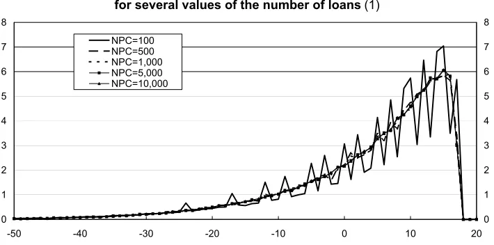
Figure 2.1 shows the return distributions for 5 portfolios which have the same char-acteristics except for the number of underlying loans. As in Krahnen and Wilde (2006)

I assume that all loans have a correlation coefficient ρ equal to 0.3, an individual default

probability of 20% and a recovery rate of 47.5%. I further assume that the risk-free interest

rate is equal to 4%. By equation (2) the coupon yield CY is equal to 18.2%. The figure

clearly shows that the return distributions of 5 portfolios with a number of loans from 100 to 10,000 are rather similar, thus proving that a fairly high level of diversification can be achieved with a relatively small number of loans. Figure 2.2 shows the cumulative distri-bution functions for the returns of the 5 portfolios, that is the probability that returns are

lower than given levels.12 _{According to the figure, the probability of incurring a loss - a}

negative return - is equal to about 30% for all portfolios and the probability of having a loss greater than 20% is about 5%. Finally, Figure 2.3 reports the VaR for a probability

level ranging from 0.1% to 10%.13

The interpretation of the figure is that, for instance, there is a 2% probability that the loss can be greater than 30% and that with probability 0.1% the loss can be greater than about 55%. It is just the case to point out that all these figures contain the same information reported in slightly different ways.

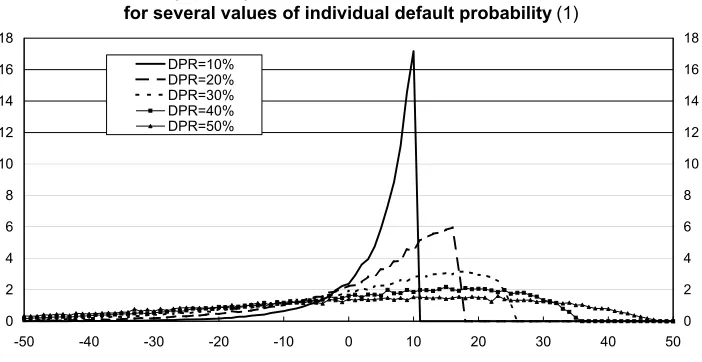
More interesting things come out when one looks at portfolios with loans that differ

in their individual default probability only.14

Figure 3.1 reports the return distribution for 5 portfolios with loans that have default probability ranging from 10% to 50%. Portfolios with greater default probabilities have return distributions with extremely fatter tails than portfolios with smaller default probabilities. This is due to the fact that greater default

12_{Formally, the figure reports the function}

F(x) =P(RP ort≤x).

13_{Formally, the figure reports the function VaR =}

F−1(x), where F is the cumulative distribution function of Figure 2.2 andxis the probability level.

14_{Assumptions on the correlation coefficient, recovery rate and risk-free interest rate are the same as}

probabilities imply not only more chances of incurring large losses but also of having very large returns when there are no defaults (because loans with greater default probability also have higher coupon yields). From Figure 3.2 it can be seen that the probability of having losses greater than 10% can range from 5% to over 30% or, said in a slightly different way, Figure 3.3 shows that when the individual default probability increases from 10% to 50% one can expect to have losses greater than 10% and 45%, respectively, with the same 5% probability.

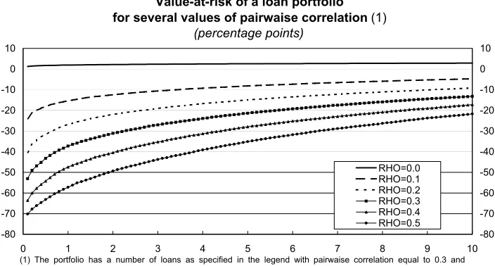
Finally, one can examine the case in which the correlation coefficientρ varies across

portfolios. 15

As shown by Figure 4.1, the effect of moving the correlation coefficient from zero - as in a perfectly diversified portfolio where all loans are independent of each other - to 50% is to transform the return distribution from a normal-like distribution to a distribution with very fat tails. Raising the correlation coefficient leads the return distribution of the portfolio to be more and more concentrated in the extremes and this effect is much greater than what can be seen in the previous case of increasing individual

default probability. In the limit case in which ρ = 1, the loans either default all together

or none defaults. In that case, there would be exactly a 20% probability that all loans default, with a return of the portfolio of -52.5% - since only the recovery rate would be received back - and a 80% probability that none of the loans defaults, so that there would be a return for the portfolio of 18.2% - the coupon yield.

To conclude this sub-section it is worth to point out that there is an important effect of the correlation coefficient on the return distribution that cannot be shown in the framework used until now, but that it is crucial for understanding the results I am just about to show on the effects of securitizing loans by issuing a CDO. Remember that in

equation (1) I assumed ρ to be a real variable defined in the interval (−1,1). However,

up to now I only analysed the effects of ρ on the return distribution of the portfolio for

some positive values of that variable. This was done because I was assuming that all loans

have the sameρ. The effects ofρ on the return distribution depend on how it affects the

behaviour of the variable Vi in equation (1) and since the common risk factor X has a

symmetric distribution with zero mean, my results would not change for, say, ρ =x and

ρ =−x. However, in the following sub-section I am going to assume that the bank can

reinvest the proceeds of the securitization in new loans that have aρdifferent from the one

of the old loans, thus creating a portfolio in which loans with different correlations with

the common risk factor coexist. In that framework the sign ofρ is going to be relevant as,

for instance, the effect of a negative return ofX on the value of a firm which is positively

correlated with it could be partially offset from the positive effects on a firm negatively

15_{The assumptions on recovery rate and risk-free interest rate are still the same as defined before and}

correlated with it.

2.3 The effects of securitization on bank stability

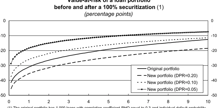
I take once again the assumptions of Krahnen and Wilde (2006) as the benchmark

case. Hence, I assume ρ= 0.3,DP = 20%,RR= 47.5% andr = 4%. The continuous line

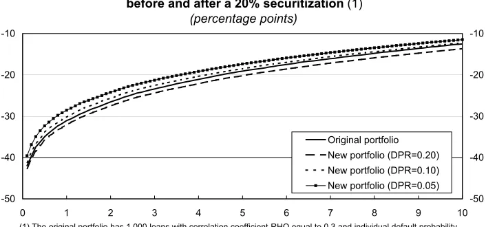
in Figure 5.1 shows the probability density function of the returns of a portfolio made of 1,000 loans with those characteristics. As shown by Krahnen and Wilde (2006), the risk for the bank of incurring large losses increases if the bank fully securitizes its portfolio by issuing a CDO of which it retains the equity tranche and reinvests the proceeds in loans with the same characteristics. This result can be seen from figures 5.2 and 5.3 through the comparison of the lines for the original portfolio with those of the case in which the loans in the new portfolio have also an individual default probability of 20%. However, if the bank reinvests the proceeds in loans of better quality, i.e. with smaller individual default probability, the overall riskiness of the bank can decrease significantly. For instance the 1% VaR goes from about -30% of the original portfolio to less than -20% of the new portfolio.

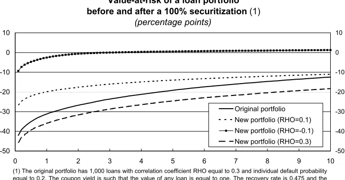
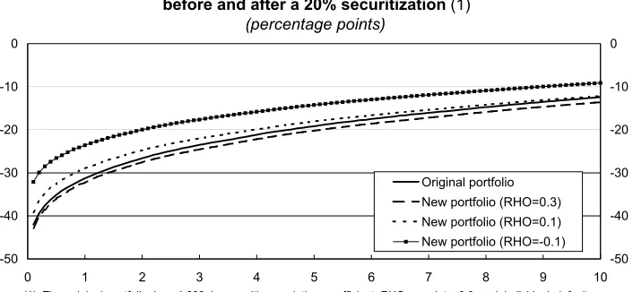
Results are even sharper if one assumes that the loans in which the proceeds of the

securitization are reinvested have a different correlation coefficient ρ. Figures 7.1 to 7.3

shows that the bank can sharply reduce its VaR for any confidence level if it reinvests in

loans with smallerρ. In the case of reinvestment in loans withρ=−0.1, for instance, the

1% VaR drop from about -30% to less than -5%. Reinvesting in loans that are negatively correlated with the common macro factor allows the bank to diversify the residual exposure to the initial portfolio, which is positively correlated with the risk factor, that it retains by holding the equity tranche of the CDO.

issuers and investors and that, of course, all results rely on the underlying assumptions.

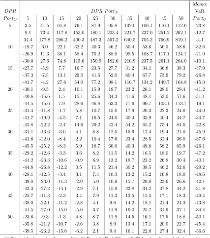
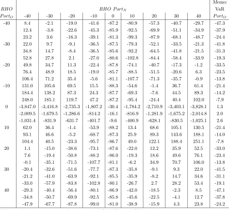
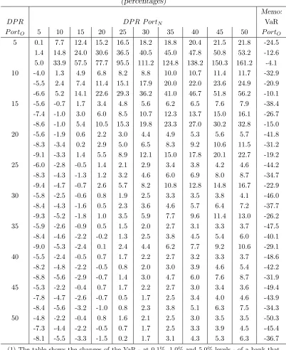
Finally, tables from 1 to 4 report VaR changes for several hypotheses about the characteristics of the loans that have been securitized and the new loans that the bank has reinvested in. Table 1, for instance, reports that 0.1%, 1% and 5% VaR, would

increase by (about) 10%, 15% and 30%, respectively, if a bank with loans withDP = 20%

securitizes them all and reinvests in loans with the same individual probability of default. However, the VaR at the same confidence level would decrease by (about) 10%, 15% and

15% if the bank reinvests in loans with DP = 10%. As a general result, Tables 1 and

2 show that a bank can reduce its VaR if it reinvests in loans with better credit quality. At the same time, the bank can reduce its VaR also by investing in loans with the same credit quality but with a different degree of correlation with the common risk factor. In particular, the VaR generally decreases when a bank with a portfolio of loans positively (negatively) correlated with the common risk factor securitizes them all and reinvests in loans which are negatively (positively) correlated with the common risk factor. Tables 3 and 4 confirm that previous results still hold if only part of the original portfolio is securitized.

3 An empirical investigation on Italian banks

In the previous section I showed that the overall riskiness of a bank can increase as well as decrease when it sells part of its loan portfolio by issuing a CDO of which it retains the equity tranche. The final results critically depend on the hypothesis one makes about the way in which the proceeds of the securitization are reinvested. The riskiness of a bank decreases every time it reinvests in loans with smaller individual default probability or in loans which are less (more) correlated with the common risk factor than the loans that have been securitized, when the correlation is positive (negative). The opposite results hold for the inverse assumptions. As a consequence of the previous analysis, it is not possible to assess the real effects of CDO issuance on banks’ risk of default on a general basis but it is necessary a case-by-case study. In this Section I provide some empirical evidence on the effects that securitization is having on Italian banks’ balance sheets and loan portfolios.

to particular categories of borrowers, or enter new markets, just because it knows that, if needed, it would be relatively easy to get rid of these new loans by securitizing them. This example is probably relevant for many American banks that in the last few years decided to increase their exposure to subprime loans.

My empirical analysis is twofold. In the first part I analyse whether the overall structure of banks’ balance sheets has been changing due to securitization. I examine broad balance sheet items to verify whether their relative shares with respect to total assets have changed during the years due to the securitization activity of the banks. The second piece of empirical analysis is instead focussed on the characteristics of single loans, and is in some sense more in line with the theoretical framework provided in the previous section. For supervisory reasons, in Italy there are very detailed loan-by-loan databases. Using those data it is possible to compare the individual probability of default of the loans that have been securitized with that of the new loans that have been granted by the same banks during the same months. Unfortunately, for reasons that will be explained later, the information in the Italian databases is not suitable for estimating whether the probability of default of the new loans is more or less correlated with that of the loans that remained in the banks’ portfolios than that of the loans that have been securitized.

3.1 Analysis of Italian bank balance sheets

I analyse the evolution of Italian bank balance sheets between 1999, the year in which the Italian law on bank loan securitization was passed, and 2007. During that period Italian banks securitized assets for 170 billion euros. About 75% of that amount was made of performing loans, that is loans not considered as troublesome by banks. Out of the 218 banks the made at least one securitization, 140 securitized only performing loans, 40 only bad loans, and 38 both types of loans. The market was rather concentrated with about a half of the total amount of securitizations made by only 10 banks (this number further reduce to 5 if one takes into account that some of them merged during the period).

I use monthly data on balance sheet items and securitizations proceeds from the Supervisory Reports to the Bank of Italy. Supervisory Reports permit to distinguish between proceeds deriving from securitization of performing and bad loans. According to Italian regulations, banks are required to classify outstanding loans to borrowers that are not expected to meet their obligations as bad loans. Clearly, this definition allows banks some degrees of discretion in judging whether a loan is bad or not. I will return on this issue later.

be-tween banks that securitized their assets and banks that did not, I use a difference-in-difference approach. In particular, I estimate pooled equations of the following type for any asset item I am interested in:

yi,t =β0+β1δt,2007+β2δi,sec+β3δi,secδt,2007+β4xi,t+ǫi,t (3)

where i= 1, . . . , N are the banks included in the sample,t∈ {1999,2007},

δt,2007=

(

0 ift= 1999

1 ift= 2007

δi,sec= (

0 if bankidid not securitize at all between 1999 and 2007

1 if bankisecuritized at least once between 1999 and 2007

and xi,t are control variables such as size, capitalization and proprietary structure.

The balance sheet items I focus on are the amount of performing loans to non-bank customers (i.e. excluding internon-bank loans and deposits to monetary authorities), bad loans to non-bank customers, loans to other subjects (i.e. banks), and securities other

than shares. 16 _{For any of those items I calculate the annual average of their monthly}

share over total assets. Given that these ratios are bounded between zero and one, I use

the logistic transformation of them as dependent variableyi,t.17 Equation (3) is estimated

using the weighted least-squares logistic regression for grouped data described in Greene (2003, pp. 686-689).

As in any difference-in-difference estimation the most interesting coefficients are

those related to the dummy variables. In particular, β1 is a measure of the average

common change of the dependent variable across all banks between 1999 and 2007,β2 is a

measure of the average difference of the dependent variable between banks that securitized

and banks that did not securitize, in both 1999 and 2007, and β3 is a measure of the

average variation of the dependent variable between 1999 and 2007 for only those banks

that securitized some of their assets. In other words, β1 captures structural changes in

the overall Italian banking system between 1999 and 2007, β2 measures those differences

that are intrinsic to banks that securitized some of their assets and that did not change

16_{Overall these items accounted for about 80% of total assets, in both 1999 and 2007. Other major items}

on the asset side of Italian banks’ balance sheets are related to repo contracts, equity and other shares, and other assets. Those items are not included in the econometric analysis because repo contracts are only used by a minority of banks (although for some of them they represent an important investment), equity and other shares are subject to non-negligible variations due to evaluation effects, and other assets represent a miscellany of sub-items whose interpretation can be not always clear.

between 1999 and 2007,18

andβ3 is a measure of how the capital structure of banks that

securitized their assets has changed. The control variables that I use are the logarithm of the annual average of total assets, an indicator of capitalization defined as the logistic transformation of the annual average of the ratio between bank’s its own capital and total asset, and a dummy variable indicating whether the bank is a mutual or cooperative bank or not.

Before running the regressions I performed a series of controls on the data. First of all, I drop data on branches of foreign banks. There are two reasons for this choice. The first one is that, due to the greater openness of the Italian banking system, there has been a huge increase of the role of foreign banks between 1999 and 2007, in terms both of numbers and total assets (from 50 to 80 and from 86 to 275 billion euros, respectively). This phenomenon is probably independent of the role of securitization in determining bank capital structures. The second reason is that for foreign banks the Italian law on securitization in 1999 did not probably represented a novelty, since for most of them it was already possible to securitize their assets in their home countries. Then, mergers and acquisitions are taken into account by considering all entities involved in these operations as a single entity for all the period taken into account (i.e. I summed the values of the corresponding balance sheet items for those banks that were involved in mergers or acquisitions). Since I use annual averages of monthly balance sheet data in my estimations, I also dropped those banks for which less than 6 monthly data are available, for either 1999 or 2007. Finally, to get rid of some outliers, I dropped 1% of observations from the

dataset (best and worst 0.5% of all balance sheet ratios).19

The final database is made of 537 banks, 80% of which are either local mutual or cooperative banks (cf. Table 5). At the end of 2007, the coverage of the sample was about 70% of all Italian banks in terms of number, total assets, loans to non-bank customers and proceeds from securitization (cf. Table 6).

The choice to restrict the analysis to just two years deserves some explanation. Indeed, it can be argued that more data with the same of higher frequency should be used. For instance one might think to use a panel of data with the time dimension being represented by all years between 1999 and 2007, and not just the first and the last year

18_{For instance, one may think that the banks that securitize their assets are also the banks that are}

technically more advanced and have better credit scoring systems. If this were true, it would be reasonable to expect that those same banks were also more prone to allow credit to non-bank customers and less to other banks or to buy less securities, since the last two types of investments generally need less sophisticated risk-management tools. Actually, in Italy the overall share of loans to non-bank customers was significantly higher for banks that securitized than for banks that did not securitize, in both 1999 and 2007.

19_{Keeping all observations does not modify signs and significance levels of the estimated coefficients, but}

of the period. One might also think to use quarterly data instead of annual data. While these are reasonable choices I nevertheless prefer to perform a comparison over a longer period of time because what I am looking for in banks’ balance sheets are structural changes only. By definition, those changes do not arise in the short-term and, more important, using higher frequency data would increase the relevance of short-term effects of the securitization process. In order make this point clearer, one can consider the case of a bank that securitizes bad loans. In a long-term perspective, the one I am interested in, it is not obvious whether such a bank should have a lower share of bad loans, just because it securitizes them, or an higher share of them, since the bank can decide to invest in riskier activities as it knows that it can easily get rid of bad loans, if needed. By using shorter term data one would only gather the mechanical effect that securitizing bad loans lead to a decrease of their share over total assets.

Table 7 shows how the balance sheet items I mentioned above changed between 1999 and 2007. Italian banks considerably increased the average share of performing loans over total assets while decreasing their loans to other banks and their investments in securities other than shares. The increase of the relative size of performing loans was common to all types of banks but was larger for banks that specialized in securitizing bad loans. For those banks the share of bad loans in their portfolios decreased by about two thirds. Banks that securitized performing loans only were also the ones with the higher share of that kind of loans in their portfolios in both 1999 and 2007. They also decreased substantially the relative size of their investments in securities other than share.

Table 8 reports the results of the econometric analysis. For performing loans, as expected from the previous review of the data, the coefficients for the both the 2007-dummy and the sec-2007-dummy are significantly positive. The first one reflects the fact that the share of performing loans over total assets grew markedly for all banks between 1999 and 2007 while the second one derives from the fact that banks that securitized had, on average, a higher share of performing loans than banks that did not securitize in both 1999 and 2007. The negative sign of the dummy variables interacting year and securitization highlights that banks that securitized had a lower growth of the share of performing loans. Negative signs on the control variables size and capitalization show that larger and more capitalized banks have lower shares of performing loans. Overall, banks that securitized some of their assets had in 2007 relatively smaller shares of both performing and bad loans and greater investments in loans to other banks and securities other than shares. These results provide support to the idea that banks that securitized their loans took that opportunity to diversify their investments in other categories of assets.

an indirect effect of securitization. If the direct effect were predominant, one should observe greater changes for those banks that securitized greater amounts of their assets. It turns out to be the case that the greatest (in absolute value) and more significant coefficients are instead predominantly associated with levels of securitization inferior to the median value. My interpretation of these results is that the indirect effects of securitization seem to have played the larger role in determining the investment choices of Italian banks. Banks that verified that they had the possibility to securitize their assets started changing their investment policies, probably under the assumption that they could quickly revert to previous policies using the instrument of securitization, if needed. On the contrary, banks that made more use of securitizations were also those who changed relatively less their policies. They have used this innovative instrument mainly has a funding resource for financing the same kind of investments. This result is coherent with Affinito and Tagliaferri (2008) who find that one of the main motivation for Italian banks to securitize their assets is to have additional resources for financing their investments.

In order to verify whether the above mentioned changes to the composition of the balance sheets have increased or decreased the overall riskiness of Italian banks one can make the following exercise. First of all, using the results of previous regressions, it

is possible to calculate the expected values of the balance sheet ratios.20

Then, one can associate to any balance sheet item a given level of expected losses and calculate an overall level of expected losses has the weighted average of the expected losses for individual items with weights equal to the predicted values of the balance sheet ratios. Table 11 reports the result of this exercise for the case in which expected losses for performing loans, bad loans, loans to banks, and securities other than shares are equal to 1%, 50%, 0.2%, and 0.4%, respectively, and losses are independent across balance sheet items. Under these assumptions, between 1999 and 2007 the levels of expected losses decreased by more than one third for banks that securitized while remained broadly unchanged for banks that did not securitize. This result is mainly driven by the fact that the share of bad loans, which represents the riskiest part of the banks’ balance sheets, dropped for banks that securitized while remaining constant for banks that did not securitize. It is interesting to note that the greatest beneficial effect is associated, once again, with banks that made less use of securitization. Those banks, in fact, were less prone to increase the share of performing loans by reducing the relatively safer investment in securities other than shares. Finally,

20_{Given that in a logistic regression for grouped data it is not possible to interpret the regression}

it is easy to verify that these results do not change qualitatively as long as one assumes, as it is reasonable, that bad loans are by far the riskiest item and that loans to banks are the safest.

3.2 Comparing securitized loans and new loans

In this section I compare, for a sample of Italian banks, the individual risk of default

of loans that have been securitized in each semestertbetween 2004 and 2007 with that of

loans that have been granted by the same banks during the same semester. In particular,

for any banki, I calculate the rate of default in semestersfor all loans that were securitized

or granted in semester t, where s is any semester betweent and the second half of 2007,

included. The rate of default is defined as the ratio between the face value, at time s,

of all loans that have been securitized or granted by iint that run into default ins and

the overall face value of loans that have been securitized or granted by i at time t. The

definition of default that I use is based on the notion of bad loan as defined by Italian regulation and I consider a borrower to be in default on all the loans she received when

at least one of those loans is classified as bad by one of her lenders.21

As already said, the definition of bad loans allows banks to have a certain degree of arbitrariness as they have to judge when the loan is likely not to be repaid. Actually, monthly default rates show a strong seasonality, probably reflecting the policies applied by major banks to review their credits. The choice to use semi-annual data relies on the need to mitigate the seasonality with which defaults are reported and also on the necessity to analyse a period of time that is long enough to allow banks to reinvest the proceeds of their securitizations but not too long to suppose that banks are doing their investments using other sources of financing only.

Section 3 showed that the characterizing features of loans for assessing riskiness of a bank are the individual probability of default and the correlation with other loans in the bank’s portfolios. However, as mentioned at the beginning of this section, I am only able to provide some empirical evidence on the first characteristic. The main reason for why it is extremely difficult to say anything on the correlation between loans that have been securitized and loans that remained in the bank’s balance sheet is the degree of arbitrariness with which Italian financial institutions can classify a loan as bad. A loan that is securitized is going to be defined as bad by the special purpose vehicle that bought it whereas loans that remain in the portfolio of the bank are going to be defined as bad by the bank itself. The fact that loans are classified as good or bad by different institutions,

21_{The reason for using this extended definition of default is based on the fact that Italian databases}

potentially using different criteria, makes the calculations of any correlation coefficient among default strongly unreliable. One possibility to circumvent this problem would be to use a sufficiently large window, say six months, that is deemed to capture most of the possible differences in the timing with which loans are classified as bad by different institutions. However, with only four years of data and semi-annual windows one would end up with at most eight couples of defaults rates (eight default rates for securitized loans and eight default rates for loans that remained in the bank’s portfolio), thus leading to estimated correlations with very high standard errors.

For my analysis I rely on two sources of data, both with loan-by-loan details. From the Italian Central Credit Register (Centrale dei Rischi) I gather data on defaults and

on loans that have been securitized. 22 _{My second source of data is the Sample Survey}

of Active and Passive Rates (Rilevazione Campionaria dei Tassi Attivi e Passivi) which contains information on new loans, and corresponding borrowers, granted from a sample

of Italian bank.23

Given that my primary interest is to know when a loan goes into default, I only take into account securitized loans that have been transferred to other institutions reporting to the Italian Central Credit Register, thus excluding foreign special purpose vehicles. I also use only data on securitizations of performing loans since, by definition, bad loans are already in default when they are transferred. Since particularly small or large loans can sometimes be treated in special ways by banks, I dropped from the dataset loans with an outstanding amount smaller than 75,000 or greater than 1,000,000 euros. Finally, for any given semester I only consider new loans granted by those banks that made at least one securitization during the same period. Overall, the final dataset includes about 493,000 new loans and about 346,000 securitized loans.

Figures 9 and 10 report the evolution over time of default rates, averaged across banks, for loans that have been securitized or granted in given semesters for the overall banking system. There are two interesting aspects in those figures. The first one is that the overall quality of new and securitized loans do not change significantly as a function of the semester in which they were granted or securitized. This result suggests the absence of an overall credit cycle during the sample period, at least when all kind of loans are taken into account and the analysis is limited to banks that used securitization to finance

22_{The Central Credit Register is a department of the Bank of Italy that collects data on borrowers}

from their lending banks. Reporting banks file detailed information for each borrower with total loans or credit lines of more than 75,000 euros. Banks are requested to report smaller exposures only in the case the borrower goes into default. Bad loans are defined on a customer basis and therefore include all the outstanding credit extended by a bank to a borrower considered insolvent.

their investments. 24

The second relevant aspect of the figures is that new loans are on average riskier than securitized loans, thus pointing to an increasing of risks for banks that securitized their assets. Overall, new loans have an average rate of default of 0.41%, significantly higher than the 0.28% of securitized loans. From the statistical point of view, the significance of the positive difference between default rates of new loans and loans that have been securitized is confirmed by Table 12, which also reports the averages of those differences across all banks for all semesters of inception (semester in which the loan was granted or securitized) and semesters of defaults. Almost all possible combinations inception/default have a positive value and many of them are statistically significant.

These results deserve a few last comments. It could be argued that one should control for other variables when comparing the riskiness of loans that have been securitized with that of new loans. Actually, it could be the case that the different riskiness of new loans with respect to securitized loans is due to the fact that the loans were granted to different sets of borrowers, with possible different credit worthiness, or had different characteristics in terms of yield (fixed or variable), maturity (shorter or longer), or whatever, that can influence the probability to run into default. It could also be argued that one should control for the time in which new and securitized loans were initially granted. In fact, Ioannidou et al. (2007) and Jim´enez et al. (2008) show that loans that are granted when interest rates are low (high) have higher (lower) probability to run into default when interest rates increase (decrease). Hence, an explanation of my results could be that securitized loans are less risky just because they were granted when interest rates were higher. While these are very interesting issues they are nonetheless outside of the scope of this paper. As shown in Section 3, what matters for the stability of a bank that securitizes its assets is the difference between the riskiness of loans that are securitized and that of new loans, no matter where that difference comes from. Whatever the reason, securitizing good loans and substituting them with loans with lower quality is not a good deal for the stability of

a bank.25

4 Conclusions

In this paper I analyse the effects of CDO issuance on the risk of default of a bank. Using Monte Carlo simulations I show that the current practice for a bank to securitize part of its loans using CDOs, of which it retains the equity tranches, and reinvest the proceeds of the securitization in other loans can increase as well decrease the risk that

24_{Bonaccorsi and Felici (2008) use a larger sample of banks to analyse mortgages to Italian households}

and find that default rates tend to rise during the same sample period.

25_{This last statement is of course subject the hypothesis that the liability side of the bank does not}

References

Affinito, M. and E. Tagliaferri (2008), “Why do banks securitize their loans? An empirical analysis on Italian Banks”, mimeo.

Altunbas, Y., L. Gambacorta and D. Marqu´es (2007), “Securitisation and the Bank Lending Channel”, Working Papers of the Bank of Italy, No. 653.

Amato, J. D. and E. M. Remolona (2003), “The Credit Spread Puzzle”, BIS Quarterly Review, December.

Bannier, C. E. and D. N. H¨ansel (2007), “Determinants of banks’ engagement in loan

securitization”, SSRN no. 1014305.

Bofondi, M. and G. Gobbi (2006), “Informational Barriers to Entry into Credit Markets”, Review of Finance, Vol. 10, pp. 39-67.

Bonaccorsi di Patti, E. and R. Felici (2008), “Il rischio dei mutui alle famiglie in Italia: evidenza da un milione di contratti”, (The risk of home mortgages in Italy: evidence from one million contracts), Occasional Papers of the Bank of Italy, No. 32 (in Italian).

Carlstrom, C. T. and K. A. Samolyk (1995), “Loan Sales as a Response to Maket-Based

Capital Constraints”, Journal of Banking and Finance, Vol. 19, pp. 627-646.

Committee on the Global Financial System (2003), “Credit Risk Transfer”, Bank for International Settlements, CGFS Pubblications, No. 20.

Cousseran, O. and I. Rahmouni (2005), “The CDO Market. Functioning and Implications in Terms of Financial Stability”, Banque de France, Financial Stability Review, June.

De Marzo, P. and D. Duffie (1999), “A Liquidity-Based Model of Security Design”, Econometrica, Vol. 67, pp. 65-99.

Duan, N. (1983), “Smearing Estimate: A Nonparametric Retransformation Method”, Journal of the American Statistical Association, Vol. 78, pp. 605-610.

FitchRatings (2006), “Global Credit Derivatives Survey: Indices Dominate Growth as

Banks’ Risk Position Shifts”,Special Report, September 21.

Franke, G. and J. P. Krahnen (2006), “Default Risk Sharing between Banks and Markets: The Contribution of Collateralized Debt Obligations”, in: The Risks of Financial Institutions, eds. M. Carey and R. Stulz, pp.603-633, University of Chicago Press.

Gorton, G. B. and G. G. Pennacchi (1995), “Banks and Loan Sales. Marketing

Nonmar-ketable Assets”, Journal of Monetary Economics, Vol. 35, pp. 389-411.

Greenspan, A. (2005), “Risk Transfer and Financial Stability”, Remarks to the Fed-eral Bank of Chicago’s Forty-first Annual Conference on Bank Structure, Chicago, Illinois, USA.

Jim´enez, G., S. Ongena, J. L. Peydr`o, and J. Saurina (2008), “Hazardous Times for

Mo-netary Policy: What do Twenty-Three Million Bank Loans Say About the Effects of Monetary Policy on Credit Risk-Taking?”, Social Science Research Network, Paper No. 1018960.

Ioannidou, V., S. Ongena, and J. L. Peydr´o (2007), “Monetary Policy and subprime

Lending: A Tall Tale of Low Federal Funds Rates, Hazardous Loan, and Reduced Loans Spreads”, mimeo.

Jiangli, W., and M. Pritsker (2008), “The Impacts of Securitization on US Bank Holding Companies”, SSRN no. 1102284.

Jiangli, W., M. Pritsker and P. Raupach (2007), “Banking and Securitization”, mimeo.

Jones, D. (2000), “Emerging Problems with the Basel Capital Accord: Regulatory

Capi-tal Arbitrage and Related Issues”,Journal of Banking and Finance, Vol. 24, pp.

35-58.

JPMorgan (1999), “The J. P. Morgan Guide to Credit Derivatives”, Published by Risk.

Krahnen, J. P. and C. Wilde (2006), “Risk Transfer with CDOs and Systemic Risk in

Banking”, CEPR Discussion Paper Series, No. 5618.

Longstaff, F. A. and A. Rajan (2006), “An Empirical Analysis of the Pricing of

Collat-eralized Debt Obligations”, NBER Working Paper Series, No. 12210.

Melennec, O. (2000), “Asset Backed Securities: A Practical Guide for Investors”, The

Appendix: The market of CDOs

Collateralized debt obligations are securities backed by the cash flows of portfolios of different financial instruments. The main characteristic of CDOs is tranching. Any CDO is actually made by several different securities, each of one has a given seniority in terms of rights on the cash flow generated by the underlying assets. Senior, mezzanine, and junior tranches rank in a decreasing order. Risks and returns offered by these tranches vary accordingly. The splitting of CDOs into different tranches dictates a sequential allocation of the losses that the underlying portfolio can incur. The most junior tranche, called equity tranche, is the first to absorb the losses deriving from one or more defaults of the assets in the underlying portfolio. If losses exceed the notional value of the equity tranche, they are absorbed by other junior and mezzanine tranches. Only if the number and the significance of defaults in the underlying portfolio are large enough senior tranches are affected and sustain the remaining part of the losses that cannot be absorbed by other tranches. The structure of the CDOs guarantees that the holders of each tranche, with the exception of the equity tranche, are protected from the risk of incurring losses by one or more other tranches. Usually, senior and mezzanine tranches are also protected by other specific credit enhancement techniques, such as overcollateralization, reserve accounts and

the trapping of excess spreads.26

Collateralized debt obligations are usually classified according to the aim of the transaction and the way in which the credit risk of the underlying portfolio is transferred.

With respect to the first dimension, one can have balance sheet CDOs and arbitrage

CDOs depending on whether the main purpose of the transaction is to modify in some

respect the composition of the balance sheet of the seller (also named originator) or to

carry out an arbitrage transaction by exploiting the potential differences between the returns required from investors on the tranches of the CDOs and the returns of the assets

included in underlying pool.27

In a balance sheet CDO the originator is usually a financial institution, most of the times a bank, that wants to get rid of some of its assets in order to have additional resources for other investments, increase the profitability, or reduce the

regulatory capital.28

Balance sheet CDOs determine a transferring of risks traditionally taken by the banking system to other investors. The aim of arbitrage CDOs is instead to carry out a market arbitrage by putting together a portfolio of assets to be used as collateral and a CDO structure such that the overall return of the underlying pool (the

26_{Melennec (2000) describes these and others credit enhancement techniques.}

27_{Carlstrom and Samolyk (1995), Gorton and Pennacchi (1995) and DeMarzo and Duffie (1999) provide}

alternative explanations for the growth in securitization activity based on the fact that certain institutions have a natural comparative advantage in originating, but not holding, illiquid assets.

28_{Jones (2000) describe many securitization techniques used by banks to reduce their regulatory capital}

arbitrageurs cash-in-flows) is greater than the overall return of the CDO’s tranches (the

arbitrageurs cash-out-flows).29

As for the ways in which credit risk can be transferred using CDOs, there are mainly

two possibilities: Either through a true sale of the assets (cash flowCDOs) or using credit

derivatives (syntheticCDOs). In a cash flow CDO the property rights on the assets in the

underlying pool are actually transferred from the originator to a special purpose vehicle

(SPV) which in turn finances the purchase using the proceeds of the issuance of the CDO. Synthetic CDOs have a more complex structure as the transferring of risk is not achieved

by the true sale of risky assets but using credit default swap (CDSs). 30

In a synthetic CDO the originator get rid of some credit risk by buying protection from the SPV using credit default swap and the SPV buys protection from the holders of the CDO tranches. If some of the underlying assets default, the originator asks the SPV to be compensated for those losses. The SPV, in turn, transfers the losses to the final investors in the CDO, according to the tranching structure. Given that there is not any initial sale of assets from the originator to the SPV, there is not even the necessity for the SPV to raise cash when issuing the CDO. That means that the buyers of the tranches of the CDO can be

required to pay nothing at the inception of the contract (unfunded syntheticCDO). They

eventually pay what they due according to the tranching structure only in case of defaults in the underlying pool. It is clear that in an unfunded CDO the ability of the SPV to compensate the originator if a credit event occurs depends on the creditworthiness of the buyers of the CDOs only. On the other hand the fact that the buyers of the CDO have

to pay nothing at inception also make this product more attractive for investors.31

In a

funded synthetic CDO, instead, final investors are required to pay the notional amount of

their tranches to the SPV which in turn invests those proceeds in high-rated bonds (usually AAA-rated government bonds) and eventually use them to compensate the originator for any loss should it suffer in the underlying pool.

Usually the overall compensation paid to CDO investors is notably smaller than the returns on the underlying assets as the difference goes to pay all the professionals that are involved in the transaction, such as originators, security firms, asset managers, trustees, rating agencies, attorneys, and accountants. Hence, one might ask why investors should buy products that return to them much less than the underlying assets. The answer is that CDOs can create customized exposures that investors desire and cannot achieve in any other way. Using CDOs it is possible to fit into investors’ various risk appetites

29_{Amato and Remolona (2003) exploit evidence from the market on arbitrage CDOs to support their}

explanation of the low level of credit spread based on the difficulty of fully diversify a credit portfolio.

30_{Roughly, in a credit default swap the seller of protection agrees to pay to the buyer of protection some}

amount of money in case of default of a reference entity, in exchange of a periodic fee.

and capital constraints. For instance less risk-adverse investors such as hedge-funds and investment banks could prefer to take an exposure in the more riskier tranches whereas pension funds and insurance companies would probably prefer to invest in more senior tranches. Collateralized debt obligations can slice the overall credit risk in the underlying portfolio into different tranches and sell each of them to the investors that feel mostly confident with the corresponding risk-return profile.

For what it has been just said, it should not be surprising if the rate of growth of CDOs issuance has been exceptionally high during the last few years, at least since the starting of the current crisis. Despite a strong decrease in the second half of the year, global issuance of CDOs in 2007 was about USD 500 trillion, more than three times greater than

in 2004 (cf. Figure 1.1).32 _{As in previous years, the bulk of the issues was represented by}

cash flow CDOs (about 70% of the total). A breakdown by purpose shows that arbitrage CDOs accounted for about 85% of total issues (cf. Figure 1.2). About 50% of total issues were backed by other structured products such as residential mortgage backed securities (RMBS), commercial mortgage backed securities (CMBS), other CDOs, CDSs, and other

securitized/structured products, and 30% were backed by high yield loans.33 _{New issues}

were mainly denominated in US dollars (70%) and euros (25%).

32_{Data are from the Securities Industry and Financial Markets Association (SIFMA), an organization}

born of the merger between The Securities Industry Association and The Bond Market Association which represents more than 650 member firms of all sizes, in all financial markets in the United States and around the world. Data do not include unfunded synthetic tranches.

33_{High yield loans are defined as transactions of borrowers with senior unsecured debt ratings below}

Tables and Figures

Figure 1.1

Global CDO market issuance data by structure(1)

(quarterly data, millions of USD)

! "

Source: Securities Industry and Financial Markets Association (SIFMA). (1) Data do not include unfunded synthetic tranches.

Figure 1.2

Global CDO market issuance data by purpose(1)

(quarterly data, millions of USD)

Source: Securities Industry and Financial Markets Association (SIFMA).

Probability density function of the returns of a loan portfolio for several values of the number of loans (1)

0 1 2 3 4 5 6 7 8

-50 -40 -30 -20 -10 0 10 20

0 1 2 3 4 5 6 7 8 NPC=100 NPC=500 NPC=1,000 NPC=5,000 NPC=10,000

(1) The portfolio has a number of loans as specified in the legend with pairwaise correlation equal to 0.3 and individual default probability equal to 0.2. The coupon yield is such that the value of any loan is equal to one. The recovery rate is 0.475 and the risk-free interest rate is 0.04.

Fig. 2.1

Cumulative distribution function of the returns of a loan portfolio for several values of the number of loans (1)

0 10 20 30 40 50 60 70 80 90 100

-50 -40 -30 -20 -10 0 10 20

0 10 20 30 40 50 60 70 80 90 100 NPC=100 NPC=500 NPC=1,000 NPC=5,000 NPC=10,000

(1) The portfolio has a number of loans as specified in the legend with pairwaise correlation equal to 0.3 and individual default probability equal to 0.2. The coupon yield is such that the value of any loan is equal to one. The recovery rate is 0.475 and the risk-free interest rate is 0.04.

Fig. 2.2

Value-at-risk of a loan portfolio for several values of the number of loans (1)

(percentage points) -60 -50 -40 -30 -20 -10

0 1 2 3 4 5 6 7 8 9 10

-60 -50 -40 -30 -20 -10 NPC=100 NPC=500 NPC=1,000 NPC=5,000 NPC=10,000

(1) The portfolio has a number of loans as specified in the legend with pairwaise correlation equal to 0.3 and individual default probability equal to 0.2. The coupon yield is such that the value of any loan is equal to one. The recovery rate is 0.475 and the risk-free interest rate is 0.04. The level of the VaR is reported in the abscissae axis in percentage points.

Probability density function of the returns of a loan portfolio for several values of individual default probability (1)

0 2 4 6 8 10 12 14 16 18

-50 -40 -30 -20 -10 0 10 20 30 40 50

0 2 4 6 8 10 12 14 16 18 DPR=10% DPR=20% DPR=30% DPR=40% DPR=50%

(1) The portfolio has 1,000 loans with pairwaise correlation equal to 0.3 and individual default probability as specified in the legend. The coupon yield is such that the value of any loan is equal to one. The recovery rate is 0.475 and the risk-free interest rate is 0.04.

Fig. 3.1

Cumulative distribution function of the returns of a loan portfolio for several values of individual default probability (1)

0 10 20 30 40 50 60 70 80 90 100

-70 -60 -50 -40 -30 -20 -10 0 10 20 30 40 50 60 70

0 10 20 30 40 50 60 70 80 90 100 DPR=10% DPR=20% DPR=30% DPR=40% DPR=50%

(1) The portfolio has 1,000 loans with pairwaise correlation equal to 0.3 and individual default probability as specified in the legend. The coupon yield is such that the value of any loan is equal to one. The recovery rate is 0.475 and the risk-free interest rate is 0.04.

Fig. 3.2

Value-at-risk of a loan portfolio

for several values of individual default probability (1) (percentage points) -70 -60 -50 -40 -30 -20 -10 0

0 1 2 3 4 5 6 7 8 9 10

-70 -60 -50 -40 -30 -20 -10 0 DPR=10% DPR=20% DPR=30% DPR=40% DPR=50%

(1) The portfolio has 1,000 loans with pairwaise correlation equal to 0.3 and individual default probability as specified in the legend. The coupon yield is such that the value of any loan is equal to one. The recovery rate is 0.475 and the risk-free interest rate is 0.04. The level of the VaR is reported in the abscissae axis in percentage points.

Probability density function of the returns of a loan portfolio for several values of pairwaise correlation (1)

0 5 10 15 20 25 30 35 40

-30 -20 -10 0 10 20

0 5 10 15 20 25 30 35 40 RHO=0.0 RHO=0.1 RHO=0.2 RHO=0.3 RHO=0.4 RHO=0.5

(1) The portfolio has 1,000 loans with pairwaise correlation as specified in the legend and individual default probability equal to 0.2. The coupon yield is such that the value of any loan is equal to one. The recovery rate is 0.475 and the risk-free interest rate is 0.04.

Fig. 4.1

Cumulative distribution function of the returns of a loan portfolio for several values of pairwaise correlation (1)

0 10 20 30 40 50 60 70 80 90 100

-60 -50 -40 -30 -20 -10 0 10 20

0 10 20 30 40 50 60 70 80 90 100 RHO=0.0 RHO=0.1 RHO=0.2 RHO=0.3 RHO=0.4 RHO=0.5

(1) The portfolio has a number of loans as specified in the legend with pairwaise correlation equal to 0.3 and individual default probability equal to 0.2. The coupon yield is such that the value of any loan is equal to one. The recovery rate is 0.475 and the risk-free interest rate is 0.04.

Fig. 4.2

Value-at-risk of a loan portfolio for several values of pairwaise correlation (1)

(percentage points) -80 -70 -60 -50 -40 -30 -20 -10 0 10

0 1 2 3 4 5 6 7 8 9 10

-80 -70 -60 -50 -40 -30 -20 -10 0 10 RHO=0.0 RHO=0.1 RHO=0.2 RHO=0.3 RHO=0.4 RHO=0.5

(1) The portfolio has a number of loans as specified in the legend with pairwaise correlation equal to 0.3 and individual default probability equal to 0.2. The coupon yield is such that the value of any loan is equal to one. The recovery rate is 0.475 and the risk-free interest rate is 0.04. The level of the VaR is reported in the abscissae axis in percentage points.

Probability density function of the returns of a loan portfolio before and after a 100% securitization (1)

0 1 2 3 4 5 6

-50 -40 -30 -20 -10 0 10 20 30

0 1 2 3 4 5 6 Original portfolio

New portfolio (DPR=0.20)

New portfolio (DPR=0.10)

New portfolio (DPR=0.05)

(1) The original portfolio has 1,000 loans with correlation coefficient RHO equal to 0.3 and individual default probability equal to 0.2. The coupon yield is such that the value of any loan is equal to one. The recovery rate is 0.475 and the risk-free interest rate is 0.04. The loans are securitized using a CDO of which the bank retains the junior tranche. The proceeds are reinvested in new loans with an individual default probability as specified in the legend.

Fig. 5.1

Cumulative distribution function of the returns of a loan portfolio before and after a 100% securitization (1)

0 10 20 30 40 50 60 70 80 90 100

-50 -40 -30 -20 -10 0 10 20 30

0 10 20 30 40 50 60 70 80 90 100 Original portfolio New portfolio (DPR=0.20) New portfolio (DPR=0.10) New portfolio (DPR=0.05)

(1) The original portfolio has 1,000 loans with correlation coefficient RHO equal to 0.3 and individual default probability equal to 0.2. The coupon yield is such that the value of any loan is equal to one. The recovery rate is 0.475 and the risk-free interest rate is 0.04. The loans are securitized using a CDO of which the bank retains the junior tranche. The proceeds are reinvested in new loans with an individual default probability as specified in the legend.

Fig. 5.2

Value-at-risk of a loan portfolio before and after a 100% securitization (1)

(percentage points) -50 -40 -30 -20 -10 0

0 1 2 3 4 5 6 7 8 9 10

-50 -40 -30 -20 -10 0 Original portfolio New portfolio (DPR=0.20) New portfolio (DPR=0.10) New portfolio (DPR=0.05)

(1) The original portfolio has 1,000 loans with correlation coefficient RHO equal to 0.3 and individual default probability equal to 0.2. The coupon yield is such that the value of any loan is equal to one. The recovery rate is 0.475 and the risk-free interest rate is 0.04. The loans are securitized using a CDO of which the bank retains the junior tranche. The proceeds are reinvested in new loans with an individual default probability as specified in the legend. The level of the VaR is reported in the abscissae axis in percentage points.