Perturbing Potential and Orbit Dynamics

Perturbing Potential and Orbit Dynamics

Javier Bootello Engineer I.C., Malaga, Spain Email: [email protected]

Received June 9, 2013; revised July 15, 2013; accepted August 6,2013

Copyright © 2013 Javier Bootello. This is an open access article distributed under the Creative Commons Attribution License, which permits unrestricted use, distribution, and reproduction in any medium, provided the original work is properly cited.

ABSTRACT

This article checks a perturbing gravitational potential, with some orbit dynamics parameters: the angular precession at each single point of any elliptic orbit, the increase of the eccentricity of the Moon and the secular increase of the Astro-nomical Unit. This potential is consistent with the solution of the precession of Mercury, event which was the first suc-cess of General Relativity, and now is near to reach its first centenary. We suggest in this paper to update the classic test of G.R., studying the gradual progression of precession, not only in its perihelion but testing a complete trajectory around the Sun.

Keywords: Gravitational Potential; Orbit Precession; Eccentricity; Astronomical Unit

1. Perturbing Gravitational Potential

P

(



)

We will set an inertial frame with the origin in the bary- centre of the Sun-Mercury system, and not in the bary- centre of the solar system; this is because we are going to examine Mercury’s orbit as a geodesic free-fall path, isolated from other planets gravitational interference.

Potential P

 

 is defined as a slight perturbation to the Newtonian gravitational potential, linked with the radial velocity of the target. We also assume potential’s transmission velocity, equal to that of light (c).

Consider a target with a radial speed Vr related to the inertial frame, moving in the same forward direction as the potential. The transit time of the potential crossing through the target, will be larger related with the transit time when the object is in a rest position and will de- crease, if they are moving in opposite directions. The larger or reduced transit time between target and poten- tial, is proportional to (Vr/c).

Be t1 the transit time of a potential crossing through an

object. If the target moves in the same forward direction as the potential, the transit time t2 will be larger than t1

and will have the following expression, only acceptable if (leaving aside second order terms in mag- nitude, as radial acceleration):

Vrc

1 Vr t c 

2 2

t c t   (1)

2 1

1

t t Vr c Vr

t c c Vr c

 _{ }







(2)

This coefficient _t₂t₁ t₁_





, is the dimensionless ra-

tio of the new real disturbing time (t2 – t1) related to the

unperturbed transit time (t1).

The new gravitational potential is equal to the Newto- nian, added with a perturbing action proportional to

2

t t t  _{2 1 1}

  . Since the potential is an energy field with

work characteristics, the perturbance is proportional to the square of time as it is the product of the acceleration by distance. The disturbance is not linear with time nor with the radial distance. It is also necessary to accept that as quantum electrodynamic iteration, the intensity is pro- portional to _



t₂t₁



t₁_2

The motion of particles in an external gravitational

field with a Maxwell framework, is in first order equiva- lent to a dynamic system linked with (v/c)2_{. [1]}

.

Perturbing potential is then defined as:

 

2 ₂

2 1

1

t t

GM GM Vr

S

r t r c

  _  _  _ _

 

 

  (3)

where  = true anomaly. (same sign as gra-

vity) for

 

0

S  

0π and S

 

 0 for π  2π

 

S

. As the Newtonian field, potential  has a clear physical basis, consistent with the laws of impulse and momentum transfer, energy conservation and the action/ reaction effect of the usual mechanics. There is not there- fore a new potential but the same classic gravitational field, perturbed by an action that increases/decreases slight- ly the force of gravity: the target has a radial speed.

 

P

 

GM

 

P S c r 2 1 GM Vr

r

  

 

S  _{ }     _{ }        

 (4)

Point out that, if we apply potential  to any per- fect sphere or any compact three-dimension target (in- stead of a single particle), the resultant ratio is three times (Vr/c)2 _{as we will conclude in Paragraph 5.}

2. Equations of Motion of Mercury Induced

by Potential

S

 



 

Any small perturbing potential applied to a target in a keplerian ellipse, produces slight changes to the orbital parameters, first of all a precession, besides other minor actions such as the increase/decrease of the orbital axis and eccentricity.

Consider   as the instantaneous angular preces- sion at each single point of the Newtonian ellipse. Pre- cession will reach a final value (Δ) at the end of one orbit as result of its gradual accumulation. We will use Landau & Lifshitz formulation [2], which defines the precession produced by a perturbing potential. This formula is valid as a theorem, suitable for any small perturbation what- ever could be its physical origin and returning the exact value. Integration is performed over an unperturbed orbit [3] (Using Langrange Planetary Equations, we reach a very similar result).

 

 _{r U}2_{ d}  _rad.

  

 

mS 0 2 2 m M M      _





(5)

where M = m h = angular momentum,

δU = perturbing potential Energy =  .

Then, the instantaneous precession referred to  is:

 

1_{r S}2

 

_rad

h h

    _  _

   ./



radians



(6)

where h = angular momentum per unit of mass.

Applied to any elliptic orbit and a planet like Mercury:

 

3 2

3 ; 1 cos GM Vr S V r c p r e sin ; eh r r p          _{ }       (7)

where e = eccentricity ; p = semi-latus

 

1 ehsin 2

pc          _{ }

2₃GM

r

h h r

      

 

sin2 2

1 cos

e h

h e p

 

 

 

 3 2 

GM c     

  (8)

derivates referred to h are:

2

1 1

e e

h h e



   [4]; (9)

and then:

 

0 d  2 ; p p h h    

 

   

 

_

(10-a)

 









_

_

2 2 2 2 2 2 0 3

sin sin cos

2 1 d

1 cos 1 cos

GM c p e e e e e               _    _       



 









2 2 2 2 0

3 sin _{2 cos d}

1 cos

GM _{e e}

c p e

_{ }          _   _     



(1 b)

 

0-







2 3 1 1 cos

cos sin sin cos

GM e c p

e e e

              

Final orbital precession Δ(2π), has the same

ever could be the eccentricity (e > 0), and is exactly the final one

(11)

value what

orbit precession of:

 

2

6

2 GM rad./orbit 43 sec.arc./cent.

c p



    (12)

The resultant one orbit precession produced turbing potential

by per-

 

S  applied to Mercury and liptic orbit, is

any el- just exactly the same precession obtained by General Relativity in 1.915, which explained the ano- maly discovered by LeVerrier in 1.859.

The question now, is how such action is achieved throughout the 88-days orbital period and what are the theoretical assumptions about the sequential and gradual progression of precession along the orbit. Potential

 

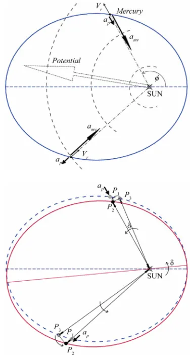
S  , and GR produce exactly the same final one orbit precession, however the equations of motion are not the same therefore, the instantaneous precession at each sin- gle point of the elliptic orbitis different. The instantane- ous precession produced by S

 

 , is not constant nor linear, causing an angular lead/lag (Ω) related to the fixed and linear GR precession.

Along the upward branch of the orbit, as Mercury moves away from the Sun, the radial velocity has the same forward direction as the gravitational potential, so perturbing acceleration increases gravity. Perturbing ac- celeration is directed inward the orbit, so Mercury will move inward in relation with the position it should oc- cupy in the keplerian ellipse.

tions (10) and (11)).

Along the descending branch of t orbit, Mercury comes closer to the Sun with a radial speed opposite to the gravitational pote

he

ntial, therefore perturbing accelera- tion, decreases gravity. The perturbing acceleration is directed outside the orbit, so Mercury will move outward in relation with the position it should occupy in the ke- plerian ellipse; the equilibrium position is located in a farther point to the Sun: a “previous” point of the cano- nical ellipse. The orbit must rotate also a forward angle: a positive instantaneous precession.

As seen in Figure 1, (graphic expression of Equations 10 and 11), the instantaneous precession  

 

produced by potential S

 

 , is always positive, producing a for-

stabl ys lo

y and a space-time with spherical sy

ward advance in both branches of the orbit. This is be- cause perturbing potential produces a e position which is alwa cated in a “previous” point in the ke- plerian trajectory (Figure 2), and therefore precession is always positive and also with symmetrical magnitude about the major axis.

[image:3.595.310.537.84.267.2]

In nearly all General Relativity textbooks and articles, the trajectory is defined starting from the Schwarzschild solution, in a geometr

Figure 1. Instantaneous (δ) and orbital (Δ) precession pro- duced by GR and S

 

 .

mmetry. On that basis, the equation of the trajectory of Mercury, and any other elliptic orbit is:

 

 

1 cos

p r

e   



  (13)

where  

 

is a small function that pro orbit differences, from the Newtonian

orbit precession. The classic relativity textbook “Gravi- by W.

duces the GR kepler-ellipse: an

tation” Misner [5], concludes in a linear progress- sion:



0



1 cos 1 2

p r

e  



 

 _   _ (14)

with 0 = 2πK

As result of it, GR instantaneous pre with a fixe related to

cession is steady, d ratio , so that the advance along rbit inear accumulation till its final value (F

ir

elliptical integral: one o , has a l

igure 1). This particular solution with a constant an- gular precession was, the f st result obtained by Ein- stein in 1915 [6]:

“...That contribution from the radius vector and de- scribed angle between the perihelion and the aphelion is obtained from the

2

1 2

d 2

x

A 3

2 2x x



  _

 

  

[image:3.595.327.515.313.664.2]



(15)

Figure 2. Instantaneous precession dynamics. Keplerian and perturbed orbit. Vr = radial velocity. anw = Newtonian

acceleration. ap = perturbing acceleration. P1 = Position in x

B B

where α1 and α2(…reciprocal values of

minimal distance from the Sun…)

GR admits also small periodic oscillations that are

the maximal and the Keplerian ellipse. P2 = Position induced by perturbing

acceleration. P3 = Equivalent position of P2 in the Keplerian

insignificant contributions and their only effect is to change slightly the position of the perihelion and the in- terpretation of rmin and e [7].

The most extended and accepted formulation of GR orbit fluctuations is: [8]

 

3 2 1 1

2 _{2 6}

c p 1 cos 2 e sin

GM _e

   _  _  _  _ (16)

 

 

 

  also produces very small oscillations but in mag- nitude, are 1/30 related with those produced by S

 



n a par- potential. There are also other prop sed i

ticular so

osals ba

lution of the Schwarzschild’s methodo-logical approaches [9].

The peak instantaneous precession produced by S

 



is at  = 1.73 rad,  = 4.56 rad, very close to the peak values of Vr (Figure 2). The maximum angular lead/lag is at  = 5.42 rad and  = 0.85 rad, with Ω = ± 0.54 rad related to the fixed and linear GR precession.

The peak positional lead/lag of Mercury, would hap- pen in A [

K 

 = 2.46 rad] and B [ = 3.82 rad]. This is because in these points, the radius is larger.

In case A, Mercury would be in a forward position regarding a GR precession. This relative position would be i = 2.4  103 _{m (transversal vector) and j = –0.36 }

103 _{m (radial vector), magnitudes which would be}

equal but with opposite sign in B. Also point out that in about 21 days, Mercury would move from the peak forward position (A) to the most delayed (B), always referred to the relative location with a constant GR precession.

Spacecraft Messenger has begun to orbit Mercury past March 18 (2011), and during two years, both will make 8.4 revolutions around the Sun. That event should after- wards allow to measure and draw accurately the geome- try of the whole orbit of Mercury, as an open geodesic free-fall path, isolated from other planets gravitational interference. Another alternative is to wait till the Bepi- Colombo be launched in 2015, an European mission to Mercury where, testing relativistic gravity is recognized as a crucial scientific objective.

3. The Increase of Eccentricity of the Orbit

of the Moon

This increase has recently been presented [10], collecting 9 lo

w

the data extracted by the Lunar Laser Ranging along 3 years since its deployment in the Moon by the Apol missions.

The increase is: (9 ± 3)  10−12_{/year [11,12].}

We will analyse the effects of a small perturbing ac- celeration over the eccentricity of any elliptic orbit. Ac- cording to Gauss Planetary Equations, (only acceptable

hen e1 and low orbit inclination), the eccentricity variation, is linked with the perturbing acceleration, what- ever could be its physical origin:

 

2

d 1 _sin

d r

e e _A

t na 



 (17)

where Ar is the radial perturbing acceleration.

The perturbing acceleration is the derivative of the per- turbing potential S

 

 related to r, th

to obtain the Newtonian acceleration from

et have the e same as we do the classic gravitational field. All the particles of the targ

same perturbing acceleration whatever they are located in the body:

 

2

2

S GM Vr

Ar

r c r r



   

   _{ }

 _{  } (18)

2 2

2 4

3 sin 1 3

1 cos

GM eh GM Vr

Ar

e c

c r

 

_{ }  _{ }

 _{ }  _{ }



  

  (19)

where Ar > 0 (same sign as gravity) for 0 π 2

r  



  and

Ar < 0 for π2π.

If we develop Equation (17) and change deriv related to time (t) with that related to

atives



2

dt d dt d d r

de_ d de  _de_ de h ₍₂₀₎

  

For a Keplerian ellipse, we have also:

 

_{ }

2

1

;

sin d

e p

na h

h

r r c p

2 2 2

2 2 2 2

sin

de h 3GM e h  p _



 _

(21)

and then,



 

2 3

2

d 3

sin d

e GM

e

c 

 

tegration will give the eccentricity increase orbit of the Moon around the Earth. Potential

(22)

The in along one

 

S  always produces a positive an

about the axis of the ellipse. If we consider the sign of Ar

in

d symmetrical effect

each branch of the orbit, we can integrate between 0 and π with a double factor.

 

2 3

orbit 2

0

6GM _{sin d}

e e

c p  





_

(23)

the definite integral is:

2 2

orbit 6GM2 4₃ 8GM2

e e e

c p c p

   

eters are: GM = 3.986  1014

 108 _m

The increase of eccentricity in one orb

12

0.279 10

e

(24)

The Earth/Moon param m3_s–2_{; e = 0.0549; a = 3.84}

it is: 

orbit  (25)

and referred to a year:

12

year _27.3365 0.279 10 3.73 10

Then, we can conclude tha

produ tential

t the increase of eccentricity of the orbit of the Moon ced by po S

 

 , is obtaine onomical detec- tion through the Lunar Laser Ranging.

4.

consistent with the data d by astr

The Increase of the Astronomical Unit

The increase of the Astronomical Unit was analysed by Krasinsky [13] however, there is not a clear explanation of its origin.

The increase is: 15 ± 4 cm/year.

Perturbing potential S

 

 produces an increase in the semi-major axis of the ellipse that, according to Gauss Planetary Equations, will have the following expres- sion:

 

2

d 2

d ₁ r

a _{e A sen}

t _n _e    (27)

Using similar formulations as in paragraph before,

 

3 3

2 2 sin

a e e

d 6

d 1

a GM

c p 

   (28)

For one orbit of the Earth around the Sun,





 

orbit 2 ₁ 2 0sin d

a e

c p e

3 3

12GM a _{ }

 





(29) 





3

_

_

orbit 2 2 2 ₂

1

16 16

1

a

GM GM

a e

c p e c

  

 _

3 2

1 e e (30)

The Earth-Sun parameters are:

GM = 13.27  1019 _m3_s–2_{; e = 0.0167}

and then:

. .year 1

U A

  1.06 cm year (31) ncrease of the Astro- nomical U

Then, we can conclude that the i

nit produced by potential S

 

 applied to the , is con t with the data obtained by astronomical detection through the a

ric measurements of distances betwee m

4], are not appropri ied to orbit of the Earth sisten

nalysis of radiomet- n the Earth and the ajor planets including observations from Martian orbit- ers from 1.971.

If we apply Gauss equations to the orbit of other plan- ets, these would be only acceptable for those with a very low eccentricity. In other cases with higher eccentricity orbits, (as Mercury), the Gauss planetary equations and others related [1 ate, appl S

 



perturbing potential. The results are:

2 Venus/orbit 0.74 10 m

a 

   ; aJupiter/orbit2.7 m;

Saturn/orbit 3.8 m a

 

5. Potential

S

 



Application to a Three

Dimension Solid Sphere

 

S is a perturbation of the classic gravitational poten-

tial due to the higher/lower pulse of time that implies a radial velocity of the target. The coefficient (Vr/c)2_{, is a}

a radial velocity

dimensionless ratio which defines the relation between the applied potential to one particle that moves with

related with another with a perfect circular orbit. Instead of a particle, we will consider a solid sphere and the perturbing potential S

 

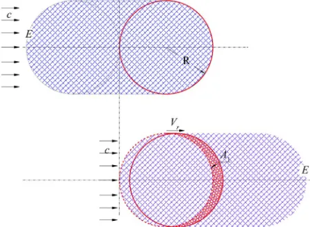
 transit action (Figure 3). The trasmission coefficient is different.

Be t1 the transit time of the potential through the equa-

torial diameter of the sphere, when the target is moving in a perfect circular orbit. When the target has a radial velocity Vr (elliptic orbit), the force of gravity associated with the potential, should produce and transmit during t1,

a larger quantity of energy-work than before; the distance travelled has been enlarge with a new length of Vr  t1

producing a very small increase of the sphere’s active volume, linked with the perturbing action: A1 Vr  t1

(Figure 3)

In order to distribute this new energy, balanced be- tween all the particles of the target, we must consider:

a) Energy (E) transmitted is in direct proportion to the spherical surface (A1).

b) Not all the diameters have the maximum length as in the equator.

c) The coefficient only compares the perturbing action regarding the initial situation.

d) Distribution of the “perturbing action” volume, be- tween the total volume of the sphere.

Therefore, the coefficient k will be:

2

1 1 1

3 3

2 3 ₃

4 3 4 3

AVrt R Vrt Vr Vr

R R



  

  ₁ (32)

and then: k 3

2R t c 

6.

Potential

Conclusions

 

P



[image:5.595.310.535.543.708.2]

 is defined as a slight perturbation to the

Newtonian gravitational potential, linked with the radial velocity of the target. The larger or reduced transit time between target and potential, is proportional to ±(Vr/c), coefficient that gives the relative increase or reduction ratio related with a particle-target in a rest position or a perfect circular movement. There is not therefore a new potential but the same classic field, perturbed by an ac- tion that increases/decreases slightly the force of gravity: the target has a radial speed.

Applied to the orbit of Mercury, produces exactly the same one orbit secular precession deduced by General Relativity; however, the equations of motion are not the same, and that means differences in the instantaneous angular precession. The instantaneous precession, could

Does these theoretic proposals suit with the complete geodesic trajectory of Mercury?

REFERENCES

[1] W. Flanders and G. Japaridze, International Journal Theo- retical Physics, Vol. 41, 2002, pp. 541-550.

doi:10.1023/A:1014257523781 [2]

[3] V. Melnikov and N. Kolosnitsyn, Gravitation & Cosmol- ogy, Vol. 10, 20

[4] G. Adkins and Review D, Vol. 75, L. Landau and M. Lifshitz, “Mekhanika,” 3rd Edition, But- terwoth-Heinemann, Oxford, 1976.

04, pp. 137-140. J. McDonnell, Physical

2007, Article ID: 082001. doi:10.1103/PhysRevD.75.082001 [5] C. Misner, K. Thorne and J. Whe

be detected by Messenger spacecraft which is now orbit-

ing Mercury and the Sun. Another alternative is to wait eler, Physics Today, Vol.

27, 1973, p. 47. doi:10.1063/1.3128805 [6] A. Einstein, “The Collected Papers of

till the BepiColombo be launched in 2015. These data should be reduced with the perturbations produced by other planets. It is certainly a difficult and complex duty but clearly available with the current development of our technology and also not expensive.

Close to reach the centenary of the formulation and first success of General Relativity, there are still some open issues.

We suggest in this paper, to update the classic test of G

A. Einstein,” Prince-

logy and Gravitation,”

, “Classical Dynamics of Par- ks, Belmont, 2004. ton University Press, Princeton, 1996.

[7] M. Berry, “Principles of Cosmo

Cambridge University Press, Cambridge, 1990. [8] B. Marion and S. Thornton

ticles and Systems,” Thomson-Broo

[9] J. Bootello, International Journal Astronomy & Astro- physics, Vol. 2, pp. 249-255.

doi:10.4236/ijaa.2012.24032

[10] J. Anderson and M. Nieto, “Astrometric

eneral Relativity, studying the gradual progression of precession, not only in its perihelion, but also along a complete trajectory around the Sun.

 

S  potential applied to the orbit of the Moon around the Earth, produces an increase of the eccentricity that is consistent with the real observed data.

 

S  potential applied to the orbit of the Earth, pro- duces an increase of the Astronomical Unit which is con- sistent with the real observed data.

Point out that it is really significant that the same gravitational potential with clear physical boundary con- ditions, consistent with the laws of impulse and momen- tu

Solar-System Ano- malies,” Proceedings of the International Astronomical Union, Vol. 5, 2010, pp. 189-197.

doi:10.1017/S1743921309990378

[11] J. Williams and D. Boggs, “Lunar Core and Mantle. What Does LLR See?” Proceedings of the 16th International Workshop on Laser Ranging, Poznan, 13-17 October 2008, pp. 101-120.

[12] L. Iorio, Royal Astronomical Society, Vol. 415, 2011, pp. 1266-1275. doi:10.1111/j.1365-2966.2011.18777.x [13] G. Krasinsky and V. Brumberg, Celestial Mechanics and

Dynamical Astronomy, Vol. 90, 2004, pp. 267-288.

m transfer, energy conservation and the action/reaction effect of the classical mechanics, could explain directly this three singularities, without any “ad hoc” parameters ar

doi:10.1007/s10569-004-0633-z

[14] J. Burns, American Journal of Physics, Vol. 44, 1976, p. 944. doi:10.1119/1.10237

rangement.

7. Appendix

 

S  potential produces a similar effect as the observe flat rota

d with spiral galaxies, d but

priate to complete the studies relate