Testing Independence for a Large Number of High–Dimensional Random Vectors

Munich Personal RePEc Archive

Testing Independence for a Large

Number of High–Dimensional Random

Vectors

Gao, Jiti and Pan, Guangming and Yang, Yanrong

Monash University, Australia, Nanyang Technological University,

Nanyang Technological University

15 March 2012

Online at

https://mpra.ub.uni-muenchen.de/45073/

Testing Independence for a Large Number of

High–Dimensional Random Vectors

Guangming Pan, Jiti Gao and Yanrong Yang

March 15, 2013

Abstract

Capturing dependence among a large number of high dimensional random vectors

is a very important and challenging problem. By arrangingnrandom vectors of length

p in the form of a matrix, we develop a linear spectral statistic of the constructed

matrix to test whether thenrandom vectors are independent or not. Specifically, the

proposed statistic can also be applied tonrandom vectors, each of whose elements can

be written as either a linear stationary process or a linear combination of a random

vector with independent elements. The asymptotic distribution of the proposed test

statistic is established in the case of 0<limn→∞ pn <∞ asn→ ∞. In order to avoid

estimating the spectrum of each random vector, a modified test statistic, which is based

on splitting the original nvectors into two equal parts and eliminating the term that

contains the inner structure of each random vector or time series, is constructed. The

facts that the limiting distribution is a normal distribution and there is no need to know

the inner structure of each investigated random vector result in simple implementation

of the constructed test statistic. Simulation results demonstrate that the proposed

test is powerful against many common dependent cases. An empirical application to

detecting dependence of the closed prices from several stocks in S&P500 also illustrates

the applicability and effectiveness of our provided test.

Keywords: Central limit theorem, Covariance stationary time series, Empirical spectral

distribution, Independence test, Large dimensional sample covariance matrix; Linear spectral

statistics.

1

Introduction

Testing cross-sectional dependence between a large number of high–dimensional random

vec-tors attracts great interest in high dimensional statistical analysis, especially in longitudinal

data and panel data analysis (Frees (1995); Mundlak (1978); Hsiao, Pesaran and Pick (2009);

Sarafidis, Yamagata and Robertson (2009); Chen, Gao and Li (2012)). In longitudinal data

or panel data analysis, one of the key reasons of pooling the data together is to overcome

the aggregation problems that arise with dependent data in modelling the behaviour of

het-erogenous agents on the basis of the representative assumption. In multivariate time series

analysis, elucidation of various causalities between time series is vital to forecasting and

prediction. Compared with the literature focusing on detecting serial dependence within a

univariate time series, relatively few studies have been done to capture dependence between

time series (Haugh (1976); Geweke (1981); Hong (1996)). Moreover, the goal of these papers

is restricted to investigating dependence between two covariance stationary time series.

Mutual independence is difficult to test while nonlinear dependence is also not easy to

detect. Mutual independence is more demanded than pairwise independence. One

conven-tional measure of linear dependence is the correlation function, which may overlook nonlinear

dependent structures that have zero correlations, e.g. Hong (1996). Another useful tool is

to utilize the equivalence of the joint distribution and the product of the corresponding

marginal distributions under independent case (see Hong (2000); Hong (2005)). Of course,

this method can capture all kinds of dependence types since it is a sufficient and

neces-sary condition of independence. However, it is just applicable to pairwise independence

test rather than mutual independence test for a large number of high–dimensional random

vectors. Hong (1999) developed a generalized spectral density approach via the empirical

characteristic function for serial independence test of one time series. This method is also

applicable to some types of linear and nonlinear dependencies but only works for detecting

pairwise dependence.

In this paper, we propose a novel test statistic to test mutual independence for nrandom

vectors of lengthpwhen n and pare comparable. Since there aren×pobserved data

avail-able, we pool them together to form a data matrix so that some features of the data matrix

to investigate independence among the initial n random vectors can be utilized. Large

di-mensional random matrix theory then serves as a powerful tool to investigate such a matrix.

then consider the empirical spectral distribution (ESD) of the eigenvalues of the

correspond-ing sample covariance matrix S = _n1XXT, where xi, i = 1,2. . . , n are the observed n time

series, each being of lengthp, i.e. xi = (X1i, X2i, . . . , Xpi)

′

. Here we would like to point out

that there have been a substantial set of research works dealing with high dimensional data

by random matrix theory (see, for example, Ledoit and Wolf (2002), Johnstone (2001), Birke

and Dette (2005) and Yao (2012)). Our approach essentially uses the ESD of the sample

covariance matrix S for n random vectors to distinguish dependence from independence.

Our discussion covers both the case where the random vectors are n covariance stationary

time series and the case where the random vectors are vectors of linear combinations of

independent random variables.

To study the size of the proposed test we first establish the limiting spectral

distribu-tion(LSD), i.e. the limit of the ESD of the sample covariance matrixSunder the finite second

moment condition on the components. This generalizes the result of Yao (2012), which

ob-tained the LSD under the finite fourth moment condition. Moreover, for the first time we

establish a central limit theorem (CLT) for linear spectral statistics of the sample covariance

matrices whose columns are covariance stationary time series under the finite fourth moment

condition on the time series components. This CLT complements the classical result of

lin-ear spectral statistics of the sample covariance matrices of the independent random vectors

with i.i.d. components or linear independent structure (see Bai and Silverstein (2009) and

Lytova and Pastur (2009)).

As stated above, correlation functions are useful enough for describing linear dependence

but can not detect all sorts of nonlinear dependecies. To some extent, our proposed test

statistic is also based on a correlation structure, i.e. the sample covariance matrix. A

natural question is how our test performs under all sorts of dependent structures. For the

Gaussian case, the sample covariance matrix of a linear covariance stationary time series can

be written in the form of S1 = _n1T11/2YY ′

T1₁/2, where T1 is a p×p nonnegative positive

Hermitian deterministic matrix and Y is a p_×n random matrix with i.i.d. components.

If the cross–sectional dependence can be described as _n1T1₁/2YT₂Y′T1₁/2 with T₂ being an

n×n Hermitian deterministic matrix, the limit of its ESD is then given in Theorem 1.2.1

of Zhang (2006), which is different from the limit of the ESD of S1 corresponding to the

independent case. In view of this, our test is able to capture this type of dependent structure.

great attention among researchers. Spatial models and factor models are two commonly used

dependent structures. The simulation given in Section 4 below shows that the proposed test

can be applied to these two types of dependence. Finite sample simulations illustrate that

the proposed test can also detect some kinds of nonlinear dependence with zero correlations

except the “ARCH” dependence. To detect the ARCH dependence we use high power of

entries Xji instead ofXji so that the test statistic still works.

The paper is organized as follows. In Section 2, we briefly review some basic concepts

and results from large dimensional random matrix theory. Section 3 states the proposed

test statistic and the asymptotic theorems for the developed statistic, including the LSD of

the sample covariance matrix for n covariance stationary time series and the CLT of the

linear spectral statistic. Section 4 analyzes the finite sample performance of the test and

investigate some kinds of commonly used cross–sectional dependent structures, including

non-zero correlation dependences(e.g. spatial models and factor models, etc.) and some

zero-correlation dependent structures. Section 5 provides an empirical application to stock

prices in S&P 500. Section 6 presents a conclusion. All the proofs are given in an appendix.

Throughout the paper, the limit is taken as n → ∞.

2

Preliminary

The observed n random vectors xi = (X1i, X2i, . . . , Xpi)

′

with i = 1,2, . . . , n are grouped

into a matrix X = (x1,x2, . . . ,xn). Denote the sample covariance matrix by

S= 1

nXX

T_{. (2.1)}

The goal is to do the following independence hypothesis test

H_{0 :x1,x2, . . . ,xn are independent; against} H_{1 :x1,x2, . . . ,xn are dependent.}

Throughout the paper, we consider two types of high dimensional random vectors xi.

The first type x_i is stationary time series specified as follows.

Assumption 1. The n time series can be expressed as

Xjt =

∞ X

k=0

where for any t = 1,2, . . . , n, _{ξi,t}∞i=−∞ is an independent and identically distributed (i.i.d)

sequence with mean zero and variance one; {bk}∞k=0 is a sequence of real numbers satisfying

P∞

k=0|bk|<∞.

This assumption covers many classical covariance stationary time series, for example, the

autoregressive (AR), moving average (MA), and autoregressive and moving average(ARMA)

time series of finite orders, etc.. In addition to ensuring stationary, the conditionP∞_k=0|bk|<

∞ is imposed to also guarantee that the spectral norm of the population covariance matrix

T₁ of each time series under investigation is bounded, as will be seen from the proof.

The second type xi is linearly generated by yi whose components are independent, as

defined below.

Assumption 2. Letxi =T11/2yiwithyi = (Y1i,· · · , Ypi)T andT11/2 being a Hermitian square

root of the nonrandom nonnegative definite Hermitian matrix T₁. For each i = 1, . . . , n,

Y1i,· · · , Ypi are i.i.d with mean zero and variance one.

Assumption 3. Let p be some function of n. Assume that n and p tend to infinity in the

same order, i.e.

c:= lim n→∞

p

n ∈(0,+∞).

When {ξi,t} are normally distributed, Assumption 1 is a special case of Assumption 2.

Indeed, it is clear that each Xjt is Gaussian distributed and eachxi is multivariate Gaussian

distribution, whose covariance matrix is a Toeplitz matrix, if{ξi,t}are normally distributed.

Thenxi in Assumption 1 can be written as a form ofT11/2yi as well. Here, to save notation,

we still useT1 as a covariance matrix ofxi although it is a Toeplitz matrix. Therefore in this

case the sample covariance matrices S associated with Assumptions 1 and 2 have a unified

expression

1

nT

1/2

1 YYTT

1/2

1 , (2.3)

where Y= (y1,· · ·,yn).

Denote the sample covariance matrix in the form of (2.3) by S₁. We are now interested

in its limiting spectral distribution (LSD) which is the limit of the empirical spectral

distri-bution(ESD) FS₁

(x). Here for any A of sizep_×p with real eigenvalues, its ESD is defined

by

FA

(x) = 1

p

p

X

j=1

where µ1 ≤ µ2 ≤ · · · ≤ µp are eigenvalues of the matrix A. A common way to find the

LSD is to first establish an equation of its Stieltjes transform, which is defined as, for any

cumulative distribution function (CDF) G(x),

mG(z) =

Z ₁

λ−zdG(λ), Im(z)6= 0.

It can be then recovered by the Frobenius-Perron formula inversion formula

G{[a, b]}= 1

πηlim→0+

Z b

a

ImmG(ζ+iη)

dζ, (2.4)

where a, bare points of continuity of G(x).

Silverstein’s result (1995) shows that the LSD of S1 in (2.3) is Fc,H(x) whose Stieltjes

transform is the unique solution to

m(z) =

Z ₁

τ1₋c₋czm(z)₋zdH(τ), (2.5)

in the set _{m _∈ C _{: −}1−c

z +cm ∈ C

+_{} if F}T₁

→ H(τ). This also yields the LSD of the sample covariance matrixSfor linear stationary processes with the Gaussian entries because

the condition that FT₁

→ H(τ) holds automatically in the case of linear stationary time series. An alternative expression of (2.5) for stationary time series will be given in the next

section by using its spectral density.

To propose a statistic to test the hypothesis H_{0 based on the feature of Fc,H(x), we}

consider an alternative that the sample covariance matrixS takes the form of

1

nT

1/2

1 YT2YTT11/2, (2.6)

where T2 is an n×n deterministic Hermitian matrix. Hence the dependence of the n time

series is described by the matrix T2.

Denote the sample covariance matrix in the form of (2.6) by S₂. Zhang (2006) provides

the LSD of the matrix S2 different from (2.5). For easy reference, we state this result in the

following lemma.

Lemma 1. In addition to Assumptions 2 and 3, we assume that as n _{→ ∞}, the ESDs

of T1 and T2, denoted by FT1 and FT2 respectively, converge weakly to two probability

non-random CDF Fc,H1,H2 with probability one, for which if H1 ≡ 1[0,+∞) or H2 ≡ 1[0,+∞),

then Fc,H1,H2 ≡1[0,+∞); otherwise if for each z ∈C

+_, 

         

s(z) = ₋z−1_(1−c)−z−1_cR 1

1+q(z)xdH2(x)

s(z) = −z−1R _1+p1_(z)ydH1(y)

s(z) = ₋z−1 _−p(z)q(z)

(2.7)

is viewed as a system of equations for the complex vector (s(z), p(z), q(z)), then the Stieltjes

transform of Fc,H1,H2, denoted by mFc,H₁,H₂(z), together with two other functions, denoted by

g1(z)and g2(z), both of which are analytic onC+, will satisfy that mFc,H₁,H₂(z), g1(z), g2(z)

is the unique solution to (2.7) in the set n

s(z), p(z), q(z) :Im s(z)>0, Im zp(z)>0, Im q(z)>0o.

From (2.5) and (2.7), we see that the LSD of the matrix S1 is different from that of

S2 since the latter one depends on the spectral distribution of the matrix T2 which is an

identity matrix under the null hypothesis H_{0. Based on the observation, a natural idea is to}

utilize the difference between the LSDs of S under H_{0 and} H_{1 to distinguish independence}

from dependence.

To this end let

Gn(λ) = p

FS

(λ)−Fcn,Hn(λ)

(2.8)

and consider the linear spectral statistic of S:

Mn =

Z

f(λ)dGn(λ), (2.9)

where Fcn,Hn(λ) is obtained from the LSD Fc,H(λ) of S under H0 and Assumptions 1 or 2 with c and H replaced by cn = p/n and Hn respectively; Hn =FT1 and f(λ) is a smooth

function. Roughly speaking, the difference between the LSDs of S under H_{0 and} H_{1 is}

reflected in behaviour of Mn. Indeed, if we rewrite the statisticMn as

ph Z f(λ)dFS

(λ)₋Fcn,Hn,H1(λ)

i

+ph Z f(λ)dFcn,Hn,H1(λ)−Fcn,Hn(λ)

i

, (2.10)

where Fcn,Hn,H1(λ) denotes the LSD of S under the alternative hypothesis H1, then we see

that the last term of (2.10) captures the difference between the LSDs ofS underH_{0 and} H_1,

not to mention the first term of (2.10). One typical example ofFcn,Hn,H1(λ) could beFc,H1,H2

in Lemma 1.

Central limit theorems (CLT) ofMn corresponding to Assumptions 1 and 2 will be given

3

Main theorems and the test statistic

3.1

Covariance stationary time series

The aim of this subsection is to establish the LSD ofSand CLT of the linear spectral statistic

Mn under the null hypothesis H0 and Assumption 1. Below we first present the LSD of S.

Theorem 1. Under Assumptions 1 and 3 and the null hypothesis H_{0, with probability one,}

the ESDFS

(x)converges to a nonrandom distribution functionFc,φ(x) whose Stieltjes

trans-form mφ(z) satisfies

z =− 1

mφ(z) + 1

2π

Z 2π

0

1

cmφ(z) + φ(λ)

−1dλ, (3.1)

where φ(λ) denotes the spectral density of xt

φ(λ) =

∞ X

k=−∞

φkeikλ, λ ∈[0,2π),

with φk =Cov(Xjt, Xj+k,t).

Remark 1. This weakens the finite fourth moment condition imposed in Yao (2012). In

addition we would point out that (3.1) is just an alternative expression of (2.5) in terms of

the spectral density ofxi. Therefore we useFc,φ(x)to denoteFc,H(x)in the case of stationary

time series.

From (3.1), we see that the Stieltjes transformmφ(z) does not have an explicit expression.

In practice, we can adopt a numerical method to calculate it which is provided in Yao (2012).

For easy reference, we state it below:

Algorithm of calculatingmφ(z): Choose an initial valuem(0)_φ (z) = u+iε, wherez =x+iε

with xa given value and ε a small enough number. Iterate the following mapping below for

k ≥0:

1

mφ(z)

=₋z+A(mφ(z)), (3.2)

where

A(mφ(z)) = 1 2π

Z 2π

0

1

cmφ(z) +φ−1(λ)

dλ,

until convergence. Let m(_φK)(z) be the final value.

We next develop CLT of Mn, which, we believe, is new in the literature. Recall the

Theorem 2. In addition to Assumptions 1 and 3, we suppose that Eξ4

j−k,t = 3. Let

f1, f2, . . . , fh be functions analytic on an open region containing the support of Fcn,Hn. Then

the random vector Z

f1(λ)dGn(λ),

Z

f2(λ)dGn(λ), . . . ,

Z

fh(λ)dGn(λ)

(3.3)

converges in distribution to a Gaussian random vector Xf1, Xf2, . . . , Xfh

with mean

func-tion for ℓ = 1,2,_{· · ·} , h,

EXfℓ =− 1 2πi

I

C

fℓ(z)

1 2π

R2π

0 cm

3

φ(z)φ2(λ) 1 +φ(λ)mφ(z)

−3

dλ

1₋c1 2π

R2π

0 m2φ(z)φ2(λ) 1 +φ(λ)mφ(z)

−2

dλ2dz

and covariance element for ℓ, r = 1,2,· · · , h,

Cov(Xfℓ, Xfr) =− 1 2π2

I

C1

I

C2

fℓ(z1)fr(z2)

m_φ(z1)−mφ(z2)

2dm_dzφ(z1) 1

dm_φ(z2)

dz2

dz1dz2. (3.4)

The contours _C above are closed and are taken in the positive direction in the complex plane,

each enclosing the support of Fc,φ(λ) and mφ(z) is the Stieltjes transform of the LSD of the

matrix S= _n1XTX.

Here m_φ(z) can be obtained from mφ(z) of (3.1) because the spectra of S differs from

that of S by_|n₋p_| zeros.

3.2

Linear independent structures

This subsection is to consider x_i satisfying Assumption 2.

The CLT of the linear spectral statisticMndefined in (2.9) has been reported in Theorem

9.10 of Bai and Silverstein (2009). For easy reference, we list it below.

Proposition 1. In addition to Assumptions 2 and 3 suppose that EY4

11 = 3 and kT1k, the spectral norm of T1, is bounded and FT₁

converges weakly to H(x). Then the random vector

(3.3) converges in distribution to a Gaussian vector with mean

EXf =− 1 2πi

I

C

f(z) c

R m3_(z)t2_dH(t)

(1+tm(z))3

1−cR m₍₁₊2(z_tm)t2₍dH_z))(2t)

2dz (3.5)

and covariance function being the same as (3.4) with m_φ(z) replaced by m(z). Here m(z),

which can be obtained fromm(z) in (2.5), is the Stieltjes transform of the LSD of the matrix

When T₁ becomes the identity matrix, H(t) becomes a degenerate distribution at point

1 and we do not need to assume that EY4

11 = 3 in this case. Theorem 1.4 of Pan and Zhou

(2008) gives CLT for the random vector (3.3). We list it below.

Proposition 2. In addition to Assumptions 2 and 3 suppose that EY4

11 < ∞. Then the random vector (3.3) converges in distribution to a Gaussian vector with mean

EXf =− 1 2πi

I

C

f(z) c m3_(z)

(1+m(z))3

1₋c₍₁₊m_tm2(₍z_z)₎₎2

2dz− c(EX

4

11−3)

2π2 I

C

f(z)

m3_(z)

(1+m(z))3

1₋c₍₁₊m_tm2(z₍)_z))dz (3.6)

and covariance

Cov(Xfl, Xfr) = − 1 π2 I C1 I C2

fl(z1)fr(z2)

(m(z1)−m(z2))2

d dz2

m(z2)

d dz1

m(z1)dz1dz2

−c(EX

4

11−3)

2π2 I

C1

I

C2

fl(z1)fr(z2)

d dz1

[ 1 1 +m(z1)

] d

dz2

[ 1 1 +m(z2)

]dz1dz2. (3.7)

3.3

Test statistic

There are two questions to be addressed before proposing a test statistic based on Theorem

2, Propositions 1 and 2. The first one is the choice of the test function f(λ) associated

with Mn in (2.9). The second one is that the mean of the asymptotic distribution of Mn,

which includes the spectral density φ(λ) of time series xi or H(x) associated with linear

independence structures, is often unknown in practice no matter what f(λ) is.

For the first question, we choose two simple test functions f1(λ) = λ and f2(λ) = λ2

for simplicity and consider their linear combination. To overcome the second difficulty, we

divide n time series into two groups, each of which contains [n/2] time series, where [n/2] is

the largest integer smaller than n/2. By Theorem 2 or Proposition 1 we have

Z

xdG(_ni)(x),

Z

x2dG(_ni)(x)−→d X_x(i), X_x(i2)

, as n→ ∞, i= 1,2, (3.8)

where G(ni)(x) = p

FS(i)

(x)−Fc

n(i),Hn(i)(x)

with cn(i) = p/[n/2], H_n(i) = H_n, F_c

n(i),Hn(i)(x) is the analogue of Fcn,Hn but corresponding to S

(i) ₌ 1

[n/2]X (i)_X(i)′

and X(i) consisting of

the i-th group of the divided time series, i = 1,2 (X = (X(1)_,X(2)_{) when n is even). Here}

Xx(i), X_x(i2)

is the limiting distribution corresponding to the i-th group time series. Since

the statistics on the left hand side of (3.8) for the two groups of time series are independent

under H0, we calculate the difference of the two statistics and obtain Z

xdGen(x),

Z

x2dGen(x)

_d

−→Xex,Xex2

where

e

Gn(x) = G(1)n (x)−G(2)n (x) =p

FS(1)(x)−FS(2)(x), (3.10)

and Xex =Xx(1)−Xx(2), Xex2 =X(1)

x2 −X

(2)

x2 .

It follows from Theorem 2 that (Xex,Xex2) is bivariate normal with mean 0 and

covari-ance matrix Ωe, where Ωe = 2Ω and Ω = (ωgh)2×2 is the asymptotic covariance matrix of

(R xdG(ni)(x),R x2dG(ni)(x)) given by

ωgh =− 1

π2 I

C1

I

C2

fg(z1)fh(z2)

(mφ(z1)−mφ(z2))2

d dz2

m_φ(z2)

d dz1

m_φ(z1)dz1dz2. (3.11)

Note that (3.10) does not involve any unknown parameters. Therefore, we propose the

following testing statistic for H_0:

Ln=

Z

xdGen(x),

Z

x2dGen(x)

e

Ω−1

  

R

xdGen(x)

R

x2_dGe

n(x)

 

. (3.12)

As for the linear independence structures, the statistic Ln is the same except thatmφ(z)

in (3.11) should be replaced by the Stieltjes transform m(z) given in Proposition 1.

The following theorem is a direct application of Theorem 2 or Proposition 1.

Theorem 3. Under the assumptions in Theorem 2 or in Proposition 1, the test statistic Ln

converges in distribution to χ2_{(2), which denotes the chi–squared random variable with the}

degree of freedom being 2.

Remark 2. The proposed statistic Ln contains the inverse covariance matrix Ωe−1 and this

matrix contains the unknown parameter m_φ(z). This parameter can be estimated either by

the algorithm provided above, or the sample Stieltjes transform m_n(z) = 1

ptr(X

′

X₋zIn)−1.

Furthermore, the asymptotic distribution is still χ2 _{after plugging in the estimator ofm}

φ(z)

by the Slutsky theorem. In view of this the proposed statistic Ln is easy to implement.

Remark 3. Traditionally, the method of dividing total samples into two parts is to use one

part to do test and the other part to estimate unknown parameters. However, the strategy

of dividing total samples into two parts here serves as a different purpose, eliminating the

unknown term involved in the linear spectral statistic Mn. Indeed, we make use of the full

strength of all observations, because if the first group and the second group are not

We also considered a Bootstrap method as follows. By a parametric bootstrap we may

redraw a sample x∗ = {x∗₁, ...,x∗_n} from the p-variate normal distribution with mean zero

and the population covariance matrix S defined in (2.1). Then consider the bootstrap linear

spectral statistic _Z

f(x)dG∗_n(x), (3.13)

where G∗

n(x) = p

h

FS₃

(x)₋Fcn,FS(x)

i

and S₃ = 1

n n

P

i=1

x∗_i(x∗_i)T_{. We can further construct a}

statistic like (3.12) by replacing Gen(x)with G∗n(x). Moreover its asymptotic distribution can

be directly obtained from Theorem 2 or Proposition 1.

However simulations show that the bootstrap statistic is not as powerful as the one

pro-posed based on the strategy of dividing observations. The key reason is that the

indepen-dence assumption under H_{0 is reflected in F}S

and its limit only such that the difference

p(FS

−Fcn,Hn) is not used. As a consequence it can not identify the alternatives whose

limit is the same as the one determined by (2.6) such as 1_nXT3XT with T3 = I+eeT (all

components of e are one).

3.4

The power under local alternatives

This section is to investigate the power for some local alternatives. The first interesting

example (local alternative) is that x1,· · · ,xn satisfy Assumption 2 butT1 there is assumed

to be random, independent of _{Yij}. Evidently,x1,· · · ,xn are not independent in this case.

Yet, Silverstein’s result (1995) indicates that (2.5) still holds if {Yij} are independent and

independent of T1. This indicates that there may be the cases where the LSD of sample

covariance matrix is also determined by (2.5) even when x1,· · · ,xn are not independent.

A nature concern is whether the statistic Ln works in this case. We now consider the case

when the random T1 is the inverse of another sample covariance matrix (S becomes the F

matrix in this case). It is then proved in Theorem 3.1 of Zheng (2012) thatLn has a central

limit theorem different from that for independent x1,· · · ,xp. The difference is caused by

randomness of T1 and one may refer to (6.32) in Step 2 of Zheng’s proof.

Although it is difficult to provide a central limi theorem for the statistic Ln for the

general alternative hypothesis H_{1, we can still evaluate the power of Ln for a class of local}

covariance matrix in the form of XT2XT, as in (2.6). Set

R(_ji) =p

Z

xidFS(j)

H₁ (x)−F

S(j)

H₀ (x)

, i= 1,2; j = 1,2; (3.14)

where FS(j)

H₀ stands for the ESD of S(j) under H0 while F

S(j)

H₁ is the ESD of S(j) under H1.

Theorem 4. In addition to assumptions in Theorem 2 or Theorem 1, suppose that in

prob-ability

lim n→∞

R(_ji)→ ∞, for any i, j. (3.15)

Then

lim

n→∞P(Ln> γ1−α|

H_{1) = 1,}

where γ1−α is the critical value of χ2 under H0 corresponding to the significance level α.

Remark 4. Suppose that each column of X satisfies either Assumption 1 or Assumption 2

and all columns are independent. Condition (3.15) is equivalent to requiring

trX(j)T(j)(X(j))Ti−trX(j)(X(j))Ti → ∞, for any i, j (3.16)

in probability, where X(j)T(j)(X(j))T _{denotes the sample covariance matrix of the jth group}

of the observations under the alternative H_{1 with T}(j) _{characterizing the dependence among}

observations, while X(j)_(X(j)₎T _{stands for the sample covariance matrix of the jth group of}

the observations under the null hypothesis H0.

If

T(j) =I+eeT,

where the elements of the vector e are all equal to one, then it is straightforward to verify

that (3.16) is true. Moreover, most of the examples given in the subsequent section satisfy

(3.16).

4

Simulation results

This section provides some simulated examples to show the finite sample performance of

the proposed test statistic Ln. To show the efficiency of our test, some classical time

se-ries models, such as MA(1), AR(1) and ARMA(1,1) processes, are considered. As for the

dependent structures, we consider some dependent structures described by MA(1) model,

AR(1) model, ARMA(1,1) model and factor model. The factor model is commonly used to

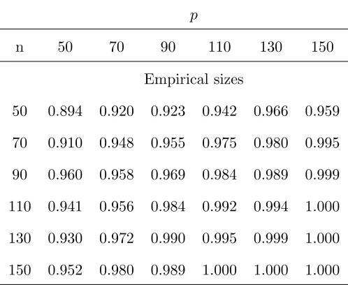
4.1

Empirical sizes and empirical powers

First we introduce the method of calculating empirical sizes and empirical powers. Since the

asymptotic distribution of the proposed test statistic Ln is a classical distribution, i.e. χ2

distribution of degree 2, the empirical sizes and powers are easy to calculate. Let z₁₋1 2α be

the 100(1−1

2α)% quantile of the asymptotic null distributionχ

2_{(2) of the test statisticL}

n.

With K replications of the data set simulated under the null hypothesis, we calculate the

empirical size as

ˆ

α= {♯ of L H

n ≥z1−1 2α}

K , (4.1)

whereLH

n represents the value of the test statisticLn based on the data simulated under the null hypothesis.

In our simulation, we choose K = 1000 as the number of repeated simulations. The

significance level is α= 0.05. Since the asymptotic null distribution of the test statistic is a

classical distribution, the quantile z₁₋1

2α is easy to know. Similarly, the empirical power is

calculated as

ˆ

β = {♯ of L A

n ≥z1−1 2α}

K , (4.2)

whereLA

n represents the value of the test statisticLn based on the data simulated under the alternative hypothesis.

4.2

Testing independence

In order to derive independent stationary time series {x_i = (X1i, X2i, . . . , Xpi)

′

: i =

1, . . . , n}, we generate data from the following three data generating processes (DGPs):

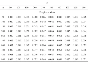
DGP1 : Xji =Zji+θ1Zj−1,i, j = 1,2, . . . , p; i= 1,2, . . . , n; (4.3)

DGP2 : Xji =φ1Xj−1,i+Zji, j = 1,2, . . . , p; i= 1,2, . . . , n; (4.4)

DGP3 : Xji−φ1Xj−1,i =Zji+θ1Zj−1,i, j = 1,2, . . . , p; i= 1,2, . . . , n, (4.5)

where {X0i, Zji :j = 1,2, . . . , p;i = 1,2, . . . , n} ∼ i.i.d N(0,1). For each DGP, we generate

p+ 100 observations and then discard the first 100 data in order to mitigate the impact of

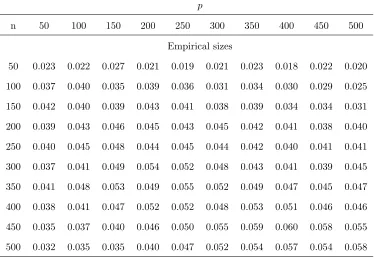
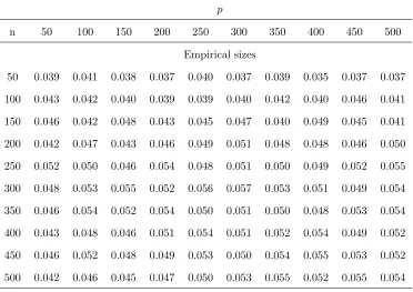
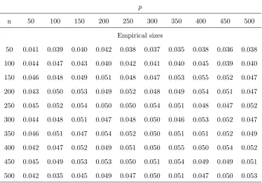
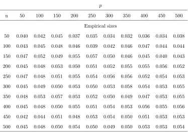
With these simulated data, we apply the proposed statisticLnand calculate the empirical

sizes. Table 1, Table 3 and Table 5 establish the empirical sizes for the three DGPs under

different pairs of (p, n). The results show that our statistic Ln works well under the null

hypothesis H_{0. Additionally, their empirical sizes from the bootstrap method proposed in}

Remark 3 are illustrated in Table 2, Table 4 and Table 6 respectively.

4.3

Testing dependence

4.3.1 Three types of correlated structures

In this section, we test four dependent structures with the proposed test and provide the

powers under each case. As in the last part of this section, we first generate data X =

(x1,x2, . . . ,xn) under DGP 1. To describe the cross-sectional dependence between xi1 and

xi2, ∀i1 6=i2, we generate new data Xe =XT, where Tis a p×p Hermitian matrix which is

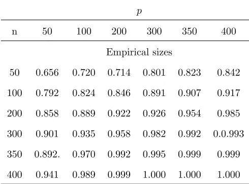
the square root of a covariance matrix. T is constructed by the following three methods.

1. MA(1) type covariance matrix Σ_{M A} = (σM A kh )

p k,h=1:

σ_kh(M A)=

          

(1 +θ2_{), k =h;}

θ, |k−h|= 1;

0, _|k₋h_|>1.

(4.6)

Under this case,T=Σ1_{M A}/2.

2. AR(1) type covariance matrix ΣAR = (σ(khAR)) p k,h=1:

σ_kh(AR) = φ

|k−h|

1₋φ2. (4.7)

Under this case,T=Σ1_AR/2.

3. ARMA(1,1) type covariance matrix ΣARM A = (σ(_khARM A))p_k,h=1:

σ(_khARM A) =

          

1 + (φ₁₋+_φθ)22, k =h;

φ+θ+(φ₁+₋θ_φ)22φ, |k−h|= 1;

φ|k−h|−1_(φ+θ+ (φ+θ)2_φ

1−φ2 ), |k−h| ≥2.

(4.8)

The powers under the three cases are illustrated in Table 7, Table 8 and Table 9. The true

parameters are taken as φ = 0.8 and θ = 0.2. It can be seen that the powers are near 1 as

n and p tend to infinity in the same order.

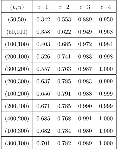
4.3.2 Factor model dependence

We consider a data generating process which comes from a dynamic factor model, which is

always used to describe cross-sectional dependence.

Xji =λ

′

fj+εji, i= 1,2, . . . , n, j = 1,2, . . . , p, (4.9)

with

fj =zj+θzj−1, i= 1,2, . . . , n, j = 1,2, . . . , p, (4.10)

where λ is an r_× 1 deterministic vector whose elements are called factor loadings; fj is an r×1 random vector generated from (4.10), whose elements are called factors and the

cross-section dependence betweenxi1 andxi2 are caused by the common factorsfj. {zj :j =

1,2, . . . , p_{} ∼}i.i.d N(0r,Ir) where 0r is an r×1 vector with elements 0 and Ir is an r×r

identity matrix. {εji :j = 1,2, . . . , p;i= 1,2, . . . , n} ∼i.i.d N(0,1) are idiosyncratic errors.

First, we generate the factor loadings in the vector λfromN(4,1) before generating data from (4.9) and (4.10). After generating the data, we can apply the proposed test statistic

Ln to the data and the empirical powers are shown in Table 10. From this table, we can

see that the powers increase as the number of factors r increases. This is reasonable in the

sense that more factors should bring in stronger dependence.

4.3.3 Common random dependence

We consider a special dependent structure which is caused by a common random part. The

data generating process is as follows.

x_i =Ay_i, i= 1,2, . . . , n, (4.11)

where A is a p _×p random matrix whose components are i.i.d standard normal random

variables; and yi, i = 1,2, . . . , n are independent p×1 random vectors, whose components

are assumed to be i.i.d standard normal random variables.

Therefore the random vectors x1,x2, . . . ,xn are dependent due to the common random

part A. The empirical powers are listed in Table 11. From the table, we can see that the

4.3.4 ARCH type dependence

It is known that dependent relations may be linear dependence or nonlinear dependence.

The examples above are all linear dependent structures. In this section, we will present a

nonlinear dependent structure.

Let us consider an autoregressive conditional heteroskedasticity (ARCH) model of the

form:

Xji =Zji

q

α0+α1Xj,i2 −1, i= 1,2, . . . , n; j = 1,2, . . . , p; (4.12)

where _{Zji : j = 1,2, . . . , p;i = 1,2, . . . , n} are white noise error terms with zero mean and

unit variance. Here we take α0, α1 ∈ (0,1) and 3α21 < 1, since the fourth moment of the

elements of Xji exists.

From this model, the sequences _{x1,x2, . . . ,xn} are dependent but uncorrelated.

More-over, this sequence is a multiple martingale difference sequence. The components of each

vector xi are independent here. This simplified assumption is imposed because the

asymp-totic theory is established for covariance time series under the assumption that the fourth

moment equals 3 while the asymptotic theorem is provided for random vectors with i.i.d.

components without this restriction.

Simulation results indicate that the proposed test statistic Ln can not detect this type

of dependence between x1,x2, . . . ,xn. Nevertheless, if we replace the elements Xjt by Xjt2,

then our statistic Ln can capture the dependence of this type. This efficiency is due to the

correlation between the high powers of _{Xjt :t= 1,2, . . . , n}.

Table 12 lists the powers of the proposed statistics Ln testing model (4.12) in several

cases, i.e. α0 andα1 take different values. From the table, we can find the phenomenon that

asα1 increases, the powers also increase. This is consistent with our intuition that largerα1

brings about larger correlation between x1,x2, . . . ,xn.

5

An empirical application

We now apply the proposed method to the daily returns of the 96 stocks from S&P500,

one of the most popular stock markets. The original data are the daily closed stock prices

of the companies belonging to S&P500 from January 2011 to December 2011, with total

derived from Wharton Research Data Services (WRDS). We use the logarithmic difference

Xji = ln(Sji/Sj−1,i). Then N = 251 logarithmic differences are available for each stock.

Note that although we have N = 251 observations available for each stock here, we only use

the firstp(p≤N) data to do the test. The value of p is comparable ton.

The interest here is to test whether the daily returns for the investigated n stocks are

dependent. Here we study three groups of companies, i.e. n = 60,70,90 stocks respectively

from S&P500. Since the distribution of Xjτ possesses high peak and heavy tails compared

with the normal distribution, which is a typical property of the financial data (Rama (2001)),

for simplicity we suppose that a transformation of the data follows a standard normal

dis-tribution,

ˆ

Xji :=

_Xji−ai

bi

βj

∼N(0,1), (5.1)

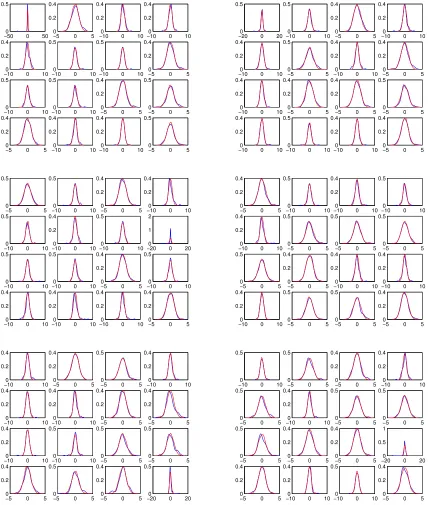
whereai, bi, βiare unknown parameters. Figure 1 illustrates the smoothed empirical densities

of the transformed data ˆXji for all the selected 96 stocks under investigation. From these

graphs, we can see that the model (5.1) is fitted well.

It is time to calculate Ln. We randomly choose n companies from the total available

96 companies and calculate the proposed statistic Ln. Repeat this experiment k = 5 times

and obtain 5 values for Ln. They are listed in Table 13. From this table, we can see that

more companies involved in the test lead to larger statistic values. For each case, all the

five statistic values are outside the interval with critical values as the end points. We should

reject the null hypothesis that the randomly chosen n= 60,70,90 stocks are independent at

the significance level 5%. This coincides with the popular financial theory that states that

cross-sectional dependence exists in modern stock markets.

6

Conclusion

This paper provides a novel approach for independence test among a large number random

vectors including covariance stationary time series of lengthpby using the empirical spectral

distribution of the sample covariance matrix of the grouped time series under investigation.

This test can capture various kinds of dependent structures, e.g. MA(1) model, AR(1)

model, ARCH(1) model and the dynamic factor model established in the simulation

sec-tion. The conventional method(LRT proposed by Anderson (1984)) utilized the correlated

instead of covariance stationary time series. Hong (1996) proposed a test statistic based

on correlation functions to investigate independence between two covariance stationary time

series. On the one hand, this idea is only efficient for normal distributed data. It may

be an inappropriate tool for non-Gaussian distributed data, such as martingale difference

sequences (e.g.ARCH(1) model), nonlinear MA(1) model etc., which possess dependent but

uncorrelated structures. On the other hand, his method is only applicable to independence

test for finite number of covariance stationary time series. Then the proposed test is more

advantageous in these two points. The simulation results and an empirical application to

cross-sectional independence test for stock prices in S&P500 highlight this approach.

7

Appendix

In this appendix, we present some lemmas and technical facts used in the proofs of the main

theorems.

7.1

Useful lemmas

Lemma 2 (Stein’s equation). Let η={ηℓ}pℓ=1 be independent Gaussian random variables of zero

mean, and Φ : Rp _→ C _{be a differentiable function with polynomially bounded partial derivatives}

Φ′_ℓ, ℓ= 1, . . . , p. Then we have

E{ηℓΦ(η)}=E{ηℓ2}E{Φ

′

ℓ(η)}, ℓ= 1, . . . , p; (7.1)

and

V ar_{Φ(η)_{} ≤} p

X

ℓ=1

E_{η2_ℓ}E_{|Φ′_ℓ(η)_|2_}. (7.2)

Lemma 3 (Generalized Stein’s equation of Lytova and Pastur (2009)). Let ηbe a random variable such thatE{|η|q+2_{}<∞ for a certain nonnegative integerq. Then for any function Φ :R→Cof}

the classCq+1 with bounded derivatives Φ(ℓ), ℓ= 1, . . . , q+ 1, we have

E_{ηΦ(η)_}= q

X

ℓ=0

κℓ+1

ℓ! E{Φ

(ℓ)_(η)}+ε

q, (7.3)

where the remainder term εq admits the bound

|ε_{q| ≤}CqE(|η|q+2) sup t∈R|

or

|ε_{q| ≤}Cq

Z 1

0

Eηq+2Φ(q+1)(ηv)(1₋v)qdv, (7.5)

with Cq ≤ 1+(3+2q) q+2

(q+1)! .

We would point out that (7.5) can be obtained from the proof of Lytova and Pastur (2009).

Our proof utilizes the generalized Fourier transform as follows:

Lemma 4 (Proposition 2.1 of Lytova and Pastur (2009)). Let g :R_{+ →} C be locally Lipshitzian and such that for someδ >0

sup t≥0

e−δt_|g(t)_|<_∞

and let _eg:{z∈C_{:Im(z)<−δ} →}C_{be its generalized Fourier transform}

e

g(z) =i−1

Z _∞

0

e−iztg(t)dt.

The inversion formula is given by

g(t) = i 2π

Z

L

eizt_eg(z)dz, t_≥0,

where L= (−∞ −iε,∞ −iε), ε > δ, and the principal value of the integral at infinity is used.

Denote the correspondence between functions and their generalized Fourier transforms asg_↔eg. Then we have

g′(t)_↔i g(+0) +z_eg(z);

Z t

0

g(τ)dτ _↔(iz)−1_eg(z);

Z t

0

g1(t−τ)g2(τ)dτ := (g1∗g2)(t)↔ieg1(z)eg2(z). (7.6)

Furthermore, we introduce a simple fact about exponential matrices below.

Lemma 5 (Duhamel formula). Let W1,W2 be n×nmatrices and t∈R. Then we have

e(W1+W2)t_=eW1t₊ Z t

0

eW1(t−s)_W

2e(W1+W2)sds. (7.7)

Moreover, if Wij(t)_1≤i,j≤n is a matrix-valued function oft∈Rthat is C∞ in the sense that each

matrix element Wij(t) is C∞. Then

d dte

W(t)₌Z 1 0

esW(t)W′(t)e(1−s)W(t)ds, (7.8)

Proof of Theorem 1: Since

E Z λdFS(λ)=E1 ptr(

1 nXX

′

)=

∞

X

k=0

b2_k,

the sequence E{FS

(λ)} is tight. By Theorem B.9 of Bai and Silverstein (2009), the proof of

Theorem 1 is complete if we can verify the following two steps:

1. For any fixed z_{∈ C}+,mn(z)−Emn(z)→0, a.s. asn→ ∞, wheremn(z) = 1_ptrG−1(z) with G−1_{(z) = (S−zI}

p)−1 and Ip being a p×p identity matrix. 2. For any fixed z_{∈ C}+_,Em

n(z)→mφ(z), asn→ ∞, wheremφ(z) =R _λ−1_zdFc,φ(λ).

The first step is omitted here, since it is similar to the proof on page 54 of Bai and Silverstein

(2009).

We will finish the second step by comparing Emn(z) for the Gaussian case and nonGaussian

case: asn→ ∞

Emn(z)−Emˆn(z)→0, (7.9)

Emˆn(z)→mφ(z), (7.10)

where ˆmn(z) is obtained from mn(z) with the elements Xjt = P∞_k=0bkξj−k,t replaced by ˆXjt =

P∞

k=0bkξˆj−k,t. Here {ξˆj−k,t}are i.i.d Gaussian random variables with mean zero and variance one

and {ξˆj−k,t}are independent of {ξj−k,t}. (7.10) obviously holds by Yao (2012).

Let Im(z) = v > 0 and below we will frequently use the fact that _|mˆn(z)| and |mn(z)| are

both bounded by 1/v without mention. We now consider (7.9) and start with the truncation of

underlying random variables. Define

Sτ = 1 nX

τ_(Xτ₎T_{, X}τ _{= (X}τ

jt)p×n, Xjtτ =

∞

X

k=0

bkξjτ−k,t, ξjτ−k,t =ξj−k,tI(|ξj−k,t| ≤τ√n), (7.11)

whereτ =τn is a positive sequence satisfying

τ _→0, 1

τE(|ξ11|

2_I(|ξ

11|> τ√n))→0. (7.12)

We claim that for every τ >0,

lim n→∞

Emn(z)−Emτn(z)

wheremτ

n(z) = 1ptrG−1τ (z) withGτ−1(z) = 1ptr(Sτ −zIp)−1. In fact, we have

Emn(z)−Emτn(z)

≤ _p√1 n

p,n

X

j,t=1

E G−_τ1(z)G−1(z)√1 nX

jt Xjt−X τ jt

+ 1 p√n

p,n

X

j,t=1

E Xjt−Xjtτ

G−1(z)G−_τ1(z)_√1 nX

jt

≤ Cnp p√n

∞

X

k=0

|b_k|E_|ξ11|I(|ξ11| ≥τ√n)≤

CE_|ξ11|2I(|ξ11| ≥τ√n)

τ

∞

X

k=0

|b_{k| →}0,

where the first inequality uses the resolvent identity

(A−zIp)−1−(B−zIp)−1 =−(A−zIp)−1(A−B)(B−zIp)−1,

holding for any Hermitian matricesA and B and the second inequality uses

G−1_τ (z)G−1(z)√1 nX

jt

≤ 1_v||G−1(z)√1 nX||=

1 v||G

−1_(z)1

nXX

T_G−1_(z)||1/2

≤ 1 v||G

−1_(z)||1/2₊1

v|z|

1/2_||G−1_{(z)|| ≤C. (7.14)}

Here k · k denotes the spectral norm of a matrix. Also throughout the paper we use C to denote

constants which may change from line to line.

In view of (7.13) it is sufficient to prove that_|Emτ

n(z)−Emˆn(z)| →0, as n→ ∞.However for simplicity below we still use notation mn(z),X, Xjt, ξj−k,t instead of using mτn(z),Xτ, Xjtτ, ξjτ−k,t and prove (7.9). But one should keep in mind that_|ξj−k,t| ≤τ√n.

We next prove (7.9) by an interpolation technique first introduced in Lytova and Pastur (2009).

To this end define the interpolation matrix

S(s) = 1

nX(s)X

T_{(s),X(s) =X} θ,t(s)

=s1/2X+ (1₋s)1/2Xˆ, s_∈[0,1] (7.15)

and

G−k(s, z) =S(s)₋zIp

−k

, mn(s, z) = 1 ptrG

−1_{(s, z), k= 1,2.}

Write Φjt(s) =

G−2(s, z)√1

nX(s)

jt. We then have

Emn(z)−Emˆn(z) =

Z 1

0

∂

∂sEmn(s, z)ds=

−1 p Z 1 0 p,n X j,t=1

Ehs−1/2√1

nXjtΦjt(s)

i

ds+1 p Z 1 0 p,n X j,t=1

Eh(1−s)−1/2√1

nXˆjtΦjt(s)

i

where we have used the formula below

∂G−1(s, z)

∂s =−G

−1_{(s, z)}∂S(s)

∂s G

−1_{(s, z).}

Consider the second term in (7.16) first. Since ˆXjt=P∞k=0bkξˆj−k,t we have

E√1

nXˆjtΦjt(s)

=

∞

X

k=0

bkE

₁

√

nξˆj−k,tΦjt(s)

. (7.17)

Applying Lemma 2 to each summand in (7.17) we have

(1₋s)−1/2

∞

X

k=0

bkE( 1 √

nξˆj−k,tΦjt(s)) = 1 n ∞ X k=0 bk p X

θ=j−k

bθ−j+kE

Dθ,t(Φjt(s))

, (7.18)

where the partial derivativeDθ,t =∂/∂(√1_nXθt(s)) and we used the fact that

∂Xˆθt ∂ξˆj−k,t

=bθ−j+k,

∂Xθt(s) ∂Xˆθt

= (1−s)1/2.

Consider the first term in (7.16) now. As before, applying the fact that Xjt =P∞_k=0bkξj−k,t and Lemma 3 to each summand of the first term in (7.16), we obtain

Es−1/2_√1

nXjtΦjt(s)

=s−1/2

∞

X

k=0

bkE

₁

√

nξj−k,tΦjt(s)

(7.19)

= s−1/2√1 n

∞

X

k=0

bkκ1,τEΦjt(s) +s−1/2 1 n

∞

X

k=0

bkκ2,τ p

X

ζ=j−k

bζ−j+kE

Dζ,t(Φjt(s))

+ε1,

whereκi,τ denotes theith cumulant of the variable ξj−k,t withi= 1,2,

|ε1| ≤

C1s−1/2

n3/2 ∞

X

k=0

|b_k|E_|ξj−k,t|3 sup |ξj−k,t|≤τ√n

|De_j2_−k,t(Φjt(s))|

,

with

e

D2_j−k,t(Φjt(s)) =Dej−k,t

_Xp

ζ=j−k

∂Φjt(s) ∂√1

nXζ,t(s) ∂√1

nXζ,t(s) ∂√1

nXζ,t ∂√1

nXζ,t ∂√1

nξj−k,t

= s p

X

ζ=j−k p

X

γ=j−k

bζ−j+kbγ−j+kDζ,t

Dγ,t(Φjt(s))

,

whereDej−k,t =∂/∂√1_nξj−k,t. Here we would point out that checking the argument of Lemma 3 in Lytova and Pastur (2009) shows that sup

t∈R

in (7.5) can be replaced by sup

|ξj−k,t|≤τ√n

in the remainder

ε1 due to the truncation step.

We conclude from (7.16)-(7.19) that

Emn(z)−Emˆn(z) =−

Z 1

0

h_s−1/2

pn1/2 ∞ X k=0 bk p,n X j,t=1

+s−1 /2 np ∞ X k=0 bk p,n X j,t=1

(κ2,τ −1) p

X

ζ=j−k

bζ−j+kE

Dζ,t(Φjt(s))

i

ds. (7.20)

The next aim is to prove that each of the three integrands goes to zero as n tends to infinity.

To this end, first let µℓ,τ(µℓ) and κℓ,τ(κℓ) be the ℓth moment and cumulant of the truncated ξjt

and the untruncated (ξjt) respectively. Then

|µℓ,τ −µℓ| ≤CE

|ξ11|ℓI(|ξ11|> τ√n)

.

As a result we have

|κℓ,τ −κℓ| ≤CE

|ξ11|ℓI(|ξ11|> τ√n)

≤ C

(τ√n)2−ℓE(|ξ11|

2_I(|ξ

11|> τ√n). (7.21)

This result uses the fact that cumulants can be expressed by moments as follows

κj =

X

λ cλµλ,

where the sum is over all additive partitions λ of the set {1, . . . , j}, {cℓ : ℓ ∈ λ} are known

coefficients and µλ =Qℓ∈λµℓ.

Second we provide the upper bound of Φjt(s), Dγ,t(Φjt(s)) and Dζ,t

Dγ,t(Φjt(s))

. For

sim-plicity, we introduce more new notation.

I(ζ, γ) =eγeTζ +eζeTγ, W(γ, t) =eγeTt 1 √

nX

T_{(s) +√}1

nX(s)ete T γ,

J1(ζ) =G−1(s, z)W(ζ, t)G−2(s, z), J2(γ, ζ) =G−1(s, z)I(γ, ζ)G−2(s, z)

J3(γ, ζ) =G−1(s, z)W(γ, t)G−2(s, z)W(ζ, t)G−1(s, z),

J4(ζ, γ) =G−1(s, z)W(ζ, t)G−1(s, z)W(γ, t)G−2(s, z),

where eγ and ej are p×1 unit vectors with the γ-th and j-th elements being 1 respectively and others being zeros; and et is n×1 a unit vector with the t-th element being 1 and others being zeros. With these notation by a simple but tedious calculation we obtain

Dγ,t(Φjt(s)) = −eTjG−2(s, z)eγ+eTjJ1(γ)

1 √

nX(s)et+e T jJT1(γ)

1 √

nX(s)et and

Dζ,t

Dγ,t(Φjt(s))

=eT_jJ1(ζ)eγ+eTjJT1(ζ)eγ−eTjJ4(ζ, γ)

1 √

nX(s)et −eT_jJ4(γ, ζ)

1 √

nX(s)et−e T

jJ3(γ, ζ)

1 √

nX(s)et+e T

jJ1(γ)eζ−eTjJT1(γ)eζ −eT_jJ3(ζ, γ)

1 √

nX(s)et−e T

jJT4(γ, ζ)

1 √

nX(s)et−e T

jJT4(ζ, γ)

1 √

nX(s)et +eT_jJ2(γ, ζ)

1 √

nX(s)et+e T

jJT2(γ, ζ)

1 √

From the expansions of Φjt(s), Dγ,t(Φjt(s)) andDζ,t

Dγ,t(Φjt(s))

we see that all the terms in

such expansions include only three factors below:

D1 =

₁

√ nX

T_(s)G−ℓ_{(s, z)√}1 nX(s)

tt, D2=

G−ℓ(s, z)√1 nX(s)

kt,

D3 =G−ℓ(s, z)_kk′, ℓ= 1,2, k, k ′

=j, ζ, or γ.

These three factors turn out to be bounded, as seen below.

Obviously |D3| ≤v−ℓ. Similar to (7.14) using

G−1(z)1

nX(s)X

T_{(s) =I+zG}−1_{(s, z). (7.22)}

one may verify that

|D2| ≤

1

vℓ−1kG−1(s, z)

1 √

nX(s)k ≤C, j = 1,2 and

|D1| ≤ k√1

nX

T_(s)G−ℓ_{(s, z)√}1

nX(s)k=kG

−ℓ_{(s, z)}1

nX(s)X

T_(s)k≤C.

Therefore Φjt(s) and the two derivatives Dγ,t(Φjt(s)), Dζ,t

Dγ,t(Φjt(s))

are bounded. This,

together with (7.21) and (7.12), yields

s−

1/2

pn1/2 ∞ X k=0 bk p,n X j,t=1

κ1,τEΦjt

≤ C

τE(|ξ11|

2_I(|ξ

11|> τ√n))→0

and _np1 ∞ X k=0 bk p,n X j,t=1

(κ2,τ −1) p

X

ζ=j−k

bζ−j+kE

Dζ,t(s)Φjt(s)≤CE(|ξ11|2I(|ξ11|> τ√n))→0.

Moreover sinceE_|ξ_jt|3 _≤τ√nand (7.12) we have

1_p p,n X j,t=1 ε1

≤Cτ →0, as n→ ∞.

These, together with (7.20), yield (7.9). The proof of this theorem is complete.

Proof of Theorem 2: The strategy of the proof is the same as that in Lytova and Pastur (2009).

That is, we first establish CLT for the case when{ξj−k,t}are i.i.dN(0,1) and then generalize it to

the general distributions.

When{ξj−k,t}are i.i.dN(0,1), as stated in Section 2, underH0, the matrixScan be written in

the form thatS= _n1T1₁/2XXT_T1/2

1 so that Theorem 9.10 of Bai and Silverstein (2009) is applicable.

asymptotic mean is obtained from that in Bai and Silverstein (2009) and the facts that (See Yao

(2012) and Gray (2009))

lim p→∞

1 p

p

X

k=1

f(σk) =

Z _∞

0

f(x)dH(x) = 1 2π

Z 2π

0

f(φ(λ))dλ.

However to apply Bai and Silverstein (2009), we have to make sure that the spectral norm of the

population covariance matrix T1 of each time series is bounded. We claim that this is ensured by

the condition P_|bj|<∞. In fact, letσk=Cov(Xjt, Xj+k,t). By the expression (2.2) of the time series and a change of variables we have

∞

X

k=0

|σ_k|=

∞

X

k=0

|Cov(

∞

X

k1=0

bk1ξj−k1,t,

∞

X

k2=0

bk2ξj+k−k2,t)|

=

∞

X

k=0

|

∞

X

k1=0

bk1bk1+k|<(

∞

X

k=0

|b_k|)2 <_∞. (7.23)

By Lemma 4.1 of Gray (2009) and (7.23) we conclude that

||T1|| ≤4 ∞

X

k=0

|σk|<∞. (7.24)

We next adopt an interpolation trick and compare the CLT of the general case with that of the

Gaussian case. Recall the definition ofGn(λ) in (2.8). Let

Nn◦[f] =

Z

f(λ)dGn(λ), Nn[f] =

Z

f(λ)dpFS(λ).

Define Nb◦

n[f] and Nnb [f] to be obtained fromNn◦[f] and Nn[f] respectively, with the entries Xjt =

P_∞

k=0bkξj−k,t replaced by ˆXjt =P∞k=0bkξˆj−k,t where{ξˆj−k,t}are i.i.d. N(0,1) and independent of

{ξj−k,t}. By the continuous theorem of characteristic functions, it suffices to show that

Rn(x) :=E

eixNn◦[f]

−EeixNbn◦[f]

→0, as n_{→ ∞}. (7.25)

Since the integrand function f admits the Fourier transform

ˆ

f(θ) = 1 2π

Z

e−iθλf(λ)dλ,

the Fourier inversion formula is

f(λ) =

Z

eiθλfˆ(θ)dθ. (7.26)

Then the statistic Nn[f] can be written as

Nn[f] =

Z

ˆ

where

un(θ) =T rU(θ), U(θ) =eiθS. (7.27)

By (7.26) we obtain

f′(S) =i

Z

ˆ

f(θ)θU(θ)dθ. (7.28)

We still use the same truncation as that in (7.11) (and use the same notation) but this time τ

satisfies (see formula (9.7.7) of Bai and Silverstein (2009))

τ _→0, τ−4E_|ξj−k,t|4I(ξj−k,t|> τ√n)→0. (7.29)

Note that

P_{X₆=Xτ_{} ≤} p,n

X

j,t=1

P_{Xjt 6=Xjt} ≤τ 1 τ4_n2

p,n X j,t=1 ∞ X k=0

bkE|ξj−k,t|4I(ξj−k,t|> τ√n)→0.

In view of this it is enough to prove that

EeixNnτ◦ [f]

−EeixNbn◦[f]

→0, as n_{→ ∞}, (7.30)

whereN◦

nτ[f] is obtained fromNn◦[f] withX replaced byXτ.

As in the proof of Theorem 1 we still use notationξj−k,t,X,Nn[f] rather thanξ_jτ_−k,t,Xτ,Nnτ◦ [f] and below prove (7.25). Recall the interpolation matrix defined in (7.15) and furthermore define

en(s, x) = exp

ixT rf S(s), U(s, θ) = (Ujk) =eiθS(s).

By (7.28) we have

Rn(x) =an

Z 1

0

∂ ∂sE

en(s, x)

ds

= ixan

Z 1

0

Ehen(s, x)T r

f′(S(s)) s−1/2√1

nX−(1−s)

−1/2_√1

nXˆ

1 √

nX τ′

(s)ids

= ₋xan

Z 1

0

ds

Z

θfˆ(θ)(Dn−Bn)dθ, (7.31)

wherean= exp(−ixR f dpFcn,φn) and

Dn= 1 √ ns p,n X j,t=1

EXjtΨjt(s)

, Bn= 1

p

n(1₋s) p,n

X

j,t=1

EXˆjtΨjt(s)

,

with

Ψjt(s) =en(s, x)

U(s, θ)√1 nX(s)

By Lemma 2 and a calculation similar to (7.17), (7.18) and (7.19) we obtain

Bn= 1 n p,n X j,t=1 ∞ X k=0 bk p X

k(1)_=j−k

b_k(1)_−j+kE

D_k(1)_t(Ψjt(s))

, (7.32)

whereD_k(1)_t=∂/∂√1_nX_k(1)_t.

Also, by Lemma 3 with q= 3 we have

Dn=

3

X

ℓ=0

Tℓτ+ε3, (7.33)

where

T0τ = s−1/2

√ n

p,n

X

j,t=1

κ1,τ

∞

X

k=0

EΨjt(s),

Tℓτ =

s(ℓ−1)/2 ℓ!n(ℓ+1)/2

p,n

X

j,t=1

κℓ+1,τ

∞ X k=0 bk p X

k(ℓ)_,k(ℓ−1)_,...,k(1)

b_k(ℓ)_−j+kb_k(ℓ−1)_−j+k· · ·b_k(1)_−j+k

·ED_k(ℓ)_tD_k(ℓ−1)_t· · ·D_k(1)_tΨjt(s)

, ℓ= 1,2,3;

and

|ε3| ≤

Cs2 n5/2

p,n X j,t=1 ∞ X k=0

|bk|

p

X

k(4)_,...,k(1)_=j−k

|b_k(4)_−j+k| · · · |b_k(1)_−j+k|

·

Z 1

0

Eh_|ξj−k,t|5Dk(4)_t· · ·D_k(1)_tΨjt(s)

ξj−k,t=vξj−k,t

i

(1₋v)3dv, (7.34)

where Ψjt(s)

ξj−k,t=vξj−k,t means thatξj−k,t involved in Ψjt(s) is replaced byvξj−k,t andκℓ,τ is the ℓth cumulant ofξj−k,t.

Next, we provide the upper bounds of derivatives:

D_k(ℓ)_tD_k(ℓ−1)_t· · ·D_k(1)_tΨjt(s), ℓ= 0,1,2,3,4.

LetY(s) = (Yrt(s)) = √1_nX(s). Applying the Duhamel formula of Lemma 4 to the entries, Ujk(ℓ),

of U(s, θ) we have

Dβα(Ujk(ℓ)) =i h

(UY(s))jα∗U_β,k(ℓ)

(θ) +(UY(s))_k(ℓ)_α∗U_jβ

(θ)i, (7.35)

where the convolution∗is defined in (7.6). Here and below we useUto denoteU(s, θ) when there is no confusion. In view of (7.35) and the fact that Ip =Ppr=1ere

′

r we have

D_k(ℓ)_t(UY(s))jt =Dk(ℓ)_{t X}p

r=1

Yrt(s)Urj

= U_k(ℓ)_j+i h

(YT(s)UY(s))tt∗Uk(ℓ)_j

(θ) +(UY(s))jt∗(UY(s))k(ℓ)_t

(θ)i,

D_k(d)_t(YT(s)UY(s))tt=Dk(d)_{t X}p

r=1

(UY(s))rtYrt(s)

= 2(UY(s))_k(d)_t+ 2i

(Yτ′(s)UY(s))tt∗(UY(s))k(d)_t

(θ), (7.37)

and by (7.28)

D_k(ℓ)_t(en(s, x)) =−2xen(s, x)

Z

θfˆ(θ)(UY(s))_k(ℓ)_tdθ, (7.38)

whereℓ, d= 1,2,3,4.

Since Pn_t=1|U_αt|2 _{= 1 and ||U||= 1, from H¨older’s inequality, we obtain}

|(UY(s))_{jt| ≤} p

X

r=1

(Yrt(s))2

1/2

, _|(YT(s)UY(s))_{tt| ≤} p

X

r=1

(Yrt(s))2. (7.39)

Recalling the definition of Ψjt(s) and repeatedly using (7.35)-(7.39) one can verify that

D_k(ℓ)_tD_k(ℓ−1)_t· · ·D_k(1)_tΨjt(s)

≤C+C p

X

r=1

(Yrt(s))2(ℓ+1)/2, ℓ= 0,1,2,3,4. (7.40)

For example see (7.49) below for the expansion of D_k(1)_tΨ_jt(s). Moreover it is straightforward

to check that ℓ = 0,1,2,3, E Pp_r=1(Yrt(s))2(ℓ+1)/2 is bounded by the fact that n2E|Yrt(s)|4 = E|Xrt(s)|4 <∞. We then conclude that

ED_k(ℓ)_tD_k(ℓ−1)_t· · ·D_k(1)_tΨjt(s)

≤Cℓ, ℓ= 0,1,2,3. (7.41)

However, to prove ε3→0, (7.40) for the caseℓ= 4 is not enough for our purpose since

E|Xrt(s)|5 ≤Cτ√n, (7.42)

not bounded. To offset this √n, one key observation is that from (7.35)-(7.38) we see that each

term in the expansion ofD_k(ℓ)_tD_k(ℓ−1)_t· · ·D_k(1)_tΨjt(s) is a product or a convolution of some of the following factors

(UY(s))h1t, (U)h2h3, (Y

T_(s)UY(s))

tt, en(s, x),

where hi can be j or any k(ℓ), ℓ = 1,· · · ,4. Let m1 and m2 be the total number of factors of

types of (UY(s))h1t and (YT(s)UY(s))tt appearing in each term of the expansion, respectively.

Then from (7.35)-(7.38) and (7.49) below we see that (m1+ 2m2)≤5 (this explains (7.40) to some

extent). Consider the case when (m1+ 2m2) = 5 first. In this case from (7.35)-(7.38) and (7.49)

below we see that at least one (UY(s))h1tmust be contained in the expansion. We below show how

to handle such terms by demonstrating one example and all other cases can be similarly proved.

Consider the term