Munich Personal RePEc Archive
Specification Tests with Weak and
Invalid Instruments
Doko Tchatoka, Firmin Sabro
School of Economics and Finance, University of Tasmania
20 July 2012
Online at
https://mpra.ub.uni-muenchen.de/40185/
Specification Tests with Weak and Invalid Instruments
∗Firmin Doko Tchatoka†
School of Economics and Finance
University of Tasmania
June 26, 2012
∗The author thanks Mardi Dunguey, Lynda Khalaf and Jean-Marie Dufour for several useful comments
and suggestions.
† School of Economics and Finance, University of Tasmania, Private Bag 85, Hobart TAS 7001,
ABSTRACT
We investigate the size of the Durbin-Wu-Hausman tests for exogeneity when instrumental
variables violate the strict exogeneity assumption. We show that these tests are severely
size distorted even for a small correlation between the structural error and instruments.
We then propose a bootstrap procedure for correcting their size. The proposed bootstrap
procedure does not require identification assumptions and is also valid even for moderate
correlations between the structural error and instruments, so it can be described as robust
to both weak and invalid instruments.
Key words: Exogeneity tests; weak instruments; instrument endogeneity; bootstrap
tech-nique.
1.
Introduction
Instrumental variables (IV) estimation can cure many ills where alternative least squares
(OLS) methods yield biased and inconsistent estimators of model coefficients. This is
espe-cially the case when explanatory variables are correlated with the error term so that OLS
estimators measure only the magnitude of association, rather than the magnitude and
direc-tion of causadirec-tion which is needed for policy analysis. IV estimadirec-tion of such models provides
a way to obtain consistent parameter estimates, once the effect of common driving variables
has been eliminated. Even though coefficients estimated in this way may have interesting
interpretations from the viewpoint of economic theory, IV procedure usually requires the
availability of exogenous instruments, at least as great as the number of coefficients to be
estimated, whereas the validity of those initial instruments is not testable. This
identify-ing indisputable exogeneity assumption has been questioned in many applied studies1. In
most IV applications, the instruments often arrive with a dark cloud of invalidity hanging
overhead and researchers usually do not know whether their correlations with the error are
exactly zero.
Concerns have intensified in recent years about the effects of instrument endogeneity
on standard inference procedures. Bound et al. (1995) provide evidence on how a slight
violation of instrument exogeneity can cause severe bias in IV estimates, especially when
identification is weak. Hausman and Hahn (2005) show that even in large-sample, the IV
estimator can have a substantial bias even when the instruments are almost uncorrelated
with the error. Recently, Chaudhuri and Rose (2009) investigate the estimation of the
ef-fect of military service on civilian earnings where both veteran status and schooling are
suspected endogenous. However, Hausman (1978) test fails to reject joint exogeneity of
both variables, though IV estimates seem larger than OLS estimates. Chaudhuri and Rose
(2009) then advocate weak instrument issues as a potential cause of the non rejection of
exogeneity. Indeed in this implication, Shea (1997)’s partial R2 statistics [see also Hall,
Rudebusch and Wilcox (1996)] are low and Stock and Yogo (2005) test suggests that the
nominal size of 5 percent Wald test for the joint significance of veteran status and schooling
is likely to be more than 25 percent. However, it may be that the non rejection of
vet-1
eran status and schooling joint exogeneity is due to the fact that some of the lottery and
proximity-to-colleges instruments used are invalid. Although the C-test and Sargan (1958)
test for instrument orthogonality confirm that over-identification restrictions are satisfied,
these tests also require the identifying assumption that at least two instruments are
indis-putably orthogonal to the error. Hence, there is still a reason for concern. Doko Tchatoka
and Dufour (2008), and Guggenberger (2011) show that inference on structural parameters
based on identification-robust statistics such as Anderson and Rubin (1949, AR-statistic),
Kleibergen (2005, KLM-statistic), and Moreira (2003, CLR-statistic), as well as their
gen-eralized empirical likelihood versions, is unreliable from the viewpoint of size control when
instruments violate “exogeneity” .
Murray (2006) [see also Samuel and Michael (2009)] suggests avoiding invalid
instru-ments in IV procedures. However, since it is difficult to test the validity of all candidate
instruments, it might seem that if we want to avoid invalid instruments, there is no hope
in trying to use IV methods. Our ultimate gaol is to show how valid inference can still be
conducted even if the strict exogeneity of the instruments is fundamentally wrong. Several
authors have recently adopted this position and this paper attempts to make a progress in
this direction. Imbens (2003) shows that bounds on average treatment effect in program
evaluation can be recovered via a sensitivity analysis of the correlations between treatment
and unobserved components of the outcomes. Ashley (2009) shows how the discrepancy
between OLS and IV estimates can be used to estimate the degree of bias under any given
assumption about the degree to which the exclusion restrictions are violated. Kiviet and
Niemczyk (2006) show that the realizations of IV estimators based on strong but invalid
instruments seem much closer to the true parameter values than those obtained from valid
but weak instruments. Imbens et al. (2011) show that consistent point estimators can
still be obtained in linear structural models with invalid instruments if the direct effects of
these instruments are uncorrelated with the effects of the instruments on the endogenous
regressors. The main findings of these studies suggest that valid inference can be conducted
even when the instruments are invalid.
In this paper, we focus on linear structural models and we wish to develop valid tests
for assessing exogeneity hypotheses allowing for a possibility that some instruments violate
to instrument endogeneity of the standard exogeneity tests of the type proposed by Durbin
(1954), Wu (1973), and Hausman (1978), henceforth DWH tests. Although DWH tests are
widely used as pretests in applied work to decide whether OLS or IV method is appropriate,
there is little evidence on how they behave when instruments violate “strict exogeneity”.
Our theoretical analysis in this paper focuses on local-to-zero invalid instruments, i.e.,
situations where the parameter which controls instrument endogeneity approaches zero at
rate [n−12] as the sample size n increases. A similar specification has been considered by
Hausman and Hahn (2005), Doko Tchatoka and Dufour (2008), Guggenberger (2011), and
Berkowitz et al. (2008). However, our simulations extend to fixed endogeneity setup, i.e.,
cases where instrument endogeneity does not depends on the sample size.
First, we provide a characterization of the limiting distribution of DWH statistics
un-der the null hypothesis of exogeneity and instrument local-to-zero invalidity. When model
identification is strong, we find (non-degenerate) asymptotic noncentral chi-square
distri-butions for all statistics, though both OLS and IV estimators are still asymptotically
con-sistent. When identification is weak, we show that the statistics converge to a mixture of
non-degenerate noncentral chi-square distributions. Therefore, the corresponding tests are
seriously size distorted whether identification is strong or weak. However, our results
indi-cate that they are more sensitive to instrument endogeneity when identification is strong
than when it is weak.
Second, we propose size correction of the tests by resorting to bootstrap techniques.
We present a Monte Carlo experiment indicating that the proposed bootstrap tests have
an overall good performance even when instrument endogeneity is moderate, so they can
be described as robust to instrument endogeneity. We apply our theoretical framework to
the trade and growth model of Frankel and Romer (1999). Our results suggest that the
instrument constructed on the basis of countries geographic characteristics in this model
is not strictly exogenous. Consequently, standard DWH tests lead to conflicting results.
However, all proposed bootstrap tests attribute the discrepancy between the OLS and 2SLS
estimates to instrument invalidity.
The remainder of this paper is organized as follows. Section 2 formulates the model and
present the statistics studied. Section 3 characterizes the asymptotic distributions of the
endogeneity through a Monte Carlo experiment. The bootstrap test procedure is presented
in Section 4, while Section 5 deals with the empirical application. Finally, Conclusions are
drawn in Section 6 and proofs are presented in the Appendix.
2.
Framework
We consider the standard linear structural model described by the following equations:
y = Xβ+u, (2.1)
X = ZΠ+V (2.2)
wherey∈Rn is a vector of observations on a dependent variable,X ∈Rn×m is a matrix of (possibly) endogenous explanatory variables,Z ∈Rn×k is a matrix of instruments (k≥m),
u= (u1, . . . , un)′∈Rnis a vector of structural disturbances,V = [V1, . . . , Vn]′ ∈Rn×m is a matrix of reduced form disturbances,β ∈Rm is an unknown structural parameter vector, while Π∈Rk×m is the unknown reduced-form coefficient matrix. Model (2.1)-(2.2) can be modified to include exogenous variables Z1. If so, our analysis will not qualitatively alter
by replacing the variables that are currently in (2.1)-(2.2) by the residuals that result from
their projection onto the space spanned by the columns of Z1.
Let ui, Vi and Zi denote the i-th row of u, V, and Z respectively, written as col-umn vectors (or scalars) and similarly for other random variables. We shall assume that
{(ui, Vi, Zi) : 1≤i≤n} is drawn i.i.d across i and the instrument matrix Z has full col-umn rank k with probability one. Our main objective is to develop inference procedures
for assessing the exogeneity of X in (2.1)-(2.2), i.e. the hypothesis
H0: cov(Xi, ui) =σXu= 0, (2.3)
taking into account that the instruments Z may be invalid, at least locally. To achieve this
goal, our approach is based essentially on DWH procedures. From that perspective, we find
2.1. DWH statistics for exogeneity
We consider the following unified formulation of DWH statistics [Doko Tchatoka and Dufour
(2011b, 2011a)]:
Tl = κl(˜β−βˆ)′Σ˜l−1(˜β−ˆβ), l= 2, 3,4, (2.4)
Hj = n(˜β−βˆ)′Σˆj−1(˜β−βˆ), j= 1,2,3 (2.5)
where Tl, l = 2,3,4, are the statistics proposed by Wu (1973, 1974), Hj, j = 1,2, 3, are three alternative Hausman (1978) type statistics, ˆβ = (X′X)−1X′y and ˜β =
(X′PZX)−1X′PZy are the OLS and IV estimators respectively,
˜
Σ2 = ˜σ22∆,ˆ Σ˜3= ˜σ2∆,ˆ Σ˜4 = ˆσ2∆,ˆ
ˆ
Σ1 = ˜σ2ΩˆIV−1−σˆ2ΩˆLS−1,Σ2ˆ = ˜σ2∆,ˆ Σ3ˆ = ˆσ2∆,ˆ
ˆ
∆ = ΩˆIV−1−ΩˆLS−1,ΩˆIV =X′PZX/n,ΩˆLS =X′X/n, ˜
σ2 = (y−Xβˆ)′(y−Xβˆ)/n,σˆ2 = (y−Xβˆ)′(y−Xβˆ)/n,
˜
σ22 = ˆσ2−(ˆβ−βˆ)′∆ˆ−1(ˆβ−βˆ),
κ2 = (n−2m)/m, and κ3=κ4 =n−m. When the instruments are strictly exogenous, all
statistics in (2.4)-(2.5) are pivotal under H0 even in finite-sample, whether identification is
strong or weak [see Doko Tchatoka and Dufour (2011b)]. Further, their pivotality in
finite-sample does not require the usual Gaussian assumption on model disturbances, i.e., the
corresponding tests remain valid in finite-sample even for non-Gaussian errors. A crucial
and relevant question is how they behave when the instruments do not satisfy the strictly
exogeneity assumption.
Our theoretical analysis in this paper considers two main setups regarding the strength
of the instruments: (A) Π is fixed with rank(Π) = m; and (B) Π = Π0/√n, where
Π0∈Rk×m is a constant matrix (possibly zero). The full rank condition ofΠ in (A) can
however be weakened to allow for partial identification2. The setup for (B) is Staiger and
Stock (1997) local-to-zero weak instrument asymptotic. In this setup, the parameter which
2
controls instrument strength approaches zero at rate [n−12] as the sample size nincreases.
2.2. Notations and model assumptions
Throughout this paper, Iq stands for the identity matrix of order q. For any full rank
n×m matrix A, PA = A(A′A)−1A is the projection matrix on the space spanned by A,
MA=In−PA.The notationvec(A) is thenm×1 dimensional column vectorization ofA andB >0 for a squared matrixB means thatB is positive definite (p.d.). The convergence
in probability is symbolized by “→p ” , “ →d ” stands for convergence in distribution while
Op(.) andop(.) denote the usual (stochastic) orders of magnitude. Finally,kUkdenotes the Euclidian norm of a vector or matrixU,i.e.,kUk= [tr(U′U)]12.
Along with the basic model (2.1)-(2.2), we shall assume the following generic
assump-tions on model variables and parameters.
Assumption 2.1 The errors {(ui, Vi) : 1≤i≤n} have zero mean and the same
nonsin-gular covariance matrix Σgiven by
Σ =
σ2u σ′V u σV u ΣV
: (m+ 1)×(m+ 1).
Furthermore, we have E(ZiZi′) =QZ >0, E[Zi(ui, Vi′)] = (σZu,0) for all i, where
σZu = d/√n (2.6)
for some constant k×1 constant vector d in Rk.
First, Assumption 2.1 requires the errors u and V to be homoskedastic. It it can
however be adapted to account for serial correlated errors. Second, while we impose Z not
be correlated with the reduced-form errors V, (2.6) implies that Z and u are correlated
when d 6= 0. However, their correlation approaches zero at rate [n−12] as the sample size
increases. Nevertheless, moderate correlations are still allowed, depending on how large
is d with respect to √n. A similar local-to-zero instrument invalidity has been used by
Berkowitz et al. (2008) [see also Doko Tchatoka and Dufour (2008) and Guggenberger
compact with the same lower and upper bounds for all instruments. Assumption 2.1 does
not require these restrictions.
Assumption 2.2 When the sample size n converges to infinity, the following convergence
results hold jointly:
(i) 1nPn
i=1(ui, Vi′)′(ui, Vi′) p
→Σ, 1nPn
i=1Zi(ui, Vi′) p
→0, n1Pn
i=1ZiZi′ p
→QZ; (ii) √1nPn
i=1(Ziui−σZu, ZiVi′, Viui−σV u) →d ψ = (ψz, ψV u), where ψz = (ψzu, ψzv),
vec(ψ) ∼ N(0,Ω), vec(ψz) ∼ N(0,Σ⊗QZ) and ψV u ∼ N(0,ΣV u) with ΣV u ≡
σ2
uΣV whenσV u= 0.
The Gaussian assumption on the limiting distributions in Assumption2.2-(ii) is implied
by Assumptions2.1 and the central limit theorem (CLT). Assumption 2.1-(ii) along with
Assumption 2.2-(ii) then entail that
1
√
n
n
X
i=1
Ziui→d ψzu+d∼N d, σ2uQZ
. (2.7)
So,Z′u/√nconverges in distribution to a Gaussian with nonzero mean ifd6= 0,thoughZ
is asymptotically uncorrelated withu hp limn→∞
Z′u
n
= 0i.
We can now examine the asymptotic behavior of the statistics in (2.4)-(2.5).
3.
Asymptotic behavior with locally invalid instruments
We now wish to analyze the sensitivity to instrument endogeneity of DWH statistics. Section
3.1 characterize their null limiting distribution when identification is strong and weak.
Section 3.2 explores the size of the corresponding tests through a Monte Carlo experiment.
3.1. Asymptotic null distributions of the statistics
To characterize the null limiting distribution of the statistics, we find useful to examine first
the sensitivity to instrument endogeneity of the vector of contrasts ˆβ −β˜ that is used in
their expressions. LemmasA.1-A.2in the Appendix present the results for both strong and
weak identification setups. The results indicate that when model identification is strong,
√
n(ˆβ −β˜) converges to a Gaussian process with nonzero mean under H0 when d 6= 0,
despite the fact that p limn→∞(ˆβ−β˜) = 0. Moreover, when identification is weak, ˆβ−β˜ converges under H0, to a mixture of Gaussian processes which have nonzero mean with
probability 1 as long as d6= 0.
We can now prove the following two results on the asymptotic behavior of the statistics.
Theorem 3.1 Suppose(2.1)-(2.2)and Assumptions2.1-2.2 are satisfied and letσυu= 0.
If further rank(Π) =m, then
T2 →d
1
mχ 2(m;
k¯τdk2),Tl
d
→χ2(m;kτ¯dk2), l= 3,4
Hj →L χ2(m;kτ¯dk2), j= 1,2,3
where τ¯d = 1
σu[(Π
′Q
ZΠ)−1−(Π′QZΠ+ΣV)−1]1/2Π′d is a k×1 constant vector.
As seen, if d 6= 0, all DWH statistics converge asymptotically to degenerate
non-central χ2 distributions under H
0. Hence, the corresponding tests are invalid (level is not
controlled) even when instrument exogeneitydis small, though both OLS and 2SLS
estima-tors are consistent in such situations when συu= 0. The magnitude of the size distortions of the tests depends on how large the non centrality parameter k¯τdk2 is. So, d may be
relatively small but the tests still exhibit large size distortions. Furthermore, as instrument
endogeneity d is unknown and difficult to estimate consistently, it is practically infeasible
to use the critical values ofχ2(m;k¯τdk2) for size correction.
Moreover, since Π[(Π′QZΠ)−1 −(Π′QZΠ+ΣV)−1]Π′ > 0, kτ¯dk2 is an increasing
function ofkdk, i.e., the size distortions of the tests increases with instrument endogeneity.
In addition, it is easy to show that k¯τdk2 ∈ [λpkdk2, λ1kdk2], where λp and λ1 are the
smallest and largest eigenvalues ofσ−2
u Π[(Π′QZΠ)−1−(Π′QZΠ+ΣV)−1]Π′, respectively. So, for a given value of instrument endogeneity d, one can establish bounds on test size
distortions through the estimates of λp and λ1.
We now derive the asymptotic null distributions of the statistics when instruments are
weak.
If furtherΠ=Π0/√n,whereΠ0 ∈Rk×m is a constant matrix(possibly zero), then we have:
T2 →d
1
m
Z
Rk×m
χ2(m;k¯νdk2)pdf(x2)dx2
T3 →d
Z
Rk×m
χ2(m; k¯νdk2)
1 +χ2(m;k¯νdk2)pdf(x2)dx2 ≤
Z
Rk×m
χ2(m;k¯νdk2)pdf(x2)dx2
T4 →d
Z
Rk×m
χ2(m;k¯νdk2)pdf(x2)dx2
H3 →L
Z
Rk×m
χ2(m;k¯νdk2)pdf(x2)dx2
Hj →d
Z
Rk×m
χ2(m; k¯ν
dk2)
1 +χ2(m;k¯νdk2)pdf(x2)dx2 ≤
Z
Rk×m
χ2(m;k¯νdk2)pdf(x2)dx2 for j= 1,2
where pdf(.) is the probability density function of ψzv and ¯νd ≡ ν¯d(x2) = σ−u1[(Π0 +
Q−Z1x2)′QZ(Π0+Q−Z1x2)]−1/2(Π0+Q−Z1x2)′d.
As indicated the above results, the statistics T2, T4 and H3 converge now to a mixture
of noncentral χ2 distributions under H
0 while the asymptotic distributions ofT3, H1, and
H2 is bounded away by a mixture of noncentral χ2 distributions. Hence, T3, H1 and H2
are less size distorted thanT2, T4 andH3. Again, we can show here that the size distortions
of all tests increase with instrument endogeneityd. An interesting question however is how
big or small the distortions are when identification is weak compare to when it is strong.
Although we do not provide a formal mathematical proof about any dominance between
both setups, it is interesting to observe that test sensitivity to instrument endogeneity is
likely more important when identification is strong than when it is weak.
To see why, consider the following two extreme situations: (1) the instruments
com-pletely irrelevant (i.e., Π0 = 0 in Theorem 3.2), and (2) they are very strong (i.e, Π is
large in Theorem3.1). For large or relatively moderate values of instrument endogeneityd,
case (2) implies large values of the non centrality parameterk¯τdk2 [see Theorem3.1] while
in case (1), the non centrality parameter kν¯0dk2 = σ−u2d′Q−Z1ψzv(ψ′zvQ−Z1ψzv)−1ψ′zvQ−Z1d [see Theorem 3.2] is bounded with probability one, independently of Π. If the mean of
kν¯0dk2 is less than k¯τdk2 with probability one (which seems highly likely to be the case
when Π is large), the tests will exhibit less size distortions in Theorem3.2 than in
Theo-rem 3.1. By the continuity of k¯νdk2 with respect to Π0, the above argument extends to
H2 are conservative when identification is weak may be viewed in some extends as an asset
for statistical inference when instruments are not strictly exogenous.
Section 3.2 illustrates our theoretical findings through a Monte Carlo experiment.
3.2. Simulation experiment
We consider a single endogenous variable model described by the following data generating
process (DGP):
y = Xβ+u, X=ZΠ+υ (3.1)
wherey and X aren×1 vectors, the errors (u, υ) are such that:
u = (1 +ρ2υ)−1/2(ε1+ρυυ) (3.2)
where (ε1i, υi)′ i.i.d∼ N(0, I2) for alli. Z containsk∈ {2,5,15}instruments each generated
i.i.d N(0,1) and its correlation with the error u is rzu ∈ {0,0.05,0.1,0.2,0.3}, where
rzu = 0 characterizes exogenous instruments while rzu 6= 0 are for invalid instruments. In particular, small values of rzu (for example rzu = 0.05) characterize locally invalid instruments. From (3.1)-(3.2), the exogeneity hypothesis of X is then expressed as H0 :
ρυ = 0. We set the true values ofβat 2 andΠ=
q
η2
nkZΠ0kΠ0, whereΠ0is a vector of ones,
η2 is the concentration parameter. Through this experiment, we varyη2 in{0,13,1000},
whereη2 ≤613 correspond to weak instruments and η2 >613 is for strong instruments [see
Hansen et al. (2008) ]. The simulations are run with sample sizesn= 100; 300, N= 10,000
replications and nominal level of 5%.
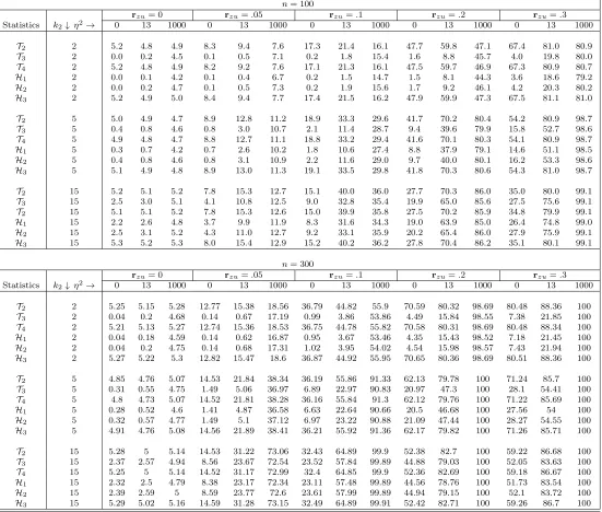
Tables 1 presents the results. When rzu= 0, i.e., when the instruments are exogenous, all DWH tests have correct level whether identification is weak (columnsη = 0; 13) or strong
(columnsη = 1000). More precisely, T2, T4 and H3 have correct size in all cases, but T3,
H1 and H2 are overly conservative when identification is weak [see also Staiger and Stock
(1997), Guggenberger (2010) and Doko Tchatoka and Dufour (2011b, 2011a)]. Now, when
rzuand the maximal rejection can be as great as 100%,suggesting that the asymptotic size of the tests converges to 1 especially when identification is strong and endogeneity fixed
(rzu 6= 0 does not dependent on the sample size). In addition, the effect of instrument endogeneity on the tests increases with model identification strength, i.e., the tests are in
general more size distorted when identification is strong (η2 = 1000) than when it is weak
(η = 0; 13), thus confirming our prior intuition. As expected, T3, H1 and H2 are less
sensitive to instrument endogeneity than T2, T4 and H3, especially when identification is
weak (see columns η= 0; 13 in the table).
Overall, our main recommendation is to use DWH tests only when we have the certitude
the instruments are strictly exogeneity. Since it is practically impossible to test the validity
of all candidate instruments, it is importance to develop tests that accounts for the violation
Table 1. Size (in %) of DWH-tests at nominal level 5%;n= 100; 300
n= 100
rzu= 0 rzu=.05 rzu=.1 rzu=.2 rzu=.3
Statistics k2↓ η2→ 0 13 1000 0 13 1000 0 13 1000 0 13 1000 0 13 1000
T2 2 5.2 4.8 4.9 8.3 9.4 7.6 17.3 21.4 16.1 47.7 59.8 47.1 67.4 81.0 80.9
T3 2 0.0 0.2 4.5 0.1 0.5 7.1 0.2 1.8 15.4 1.6 8.8 45.7 4.0 19.8 80.0
T4 2 5.2 4.8 4.9 8.2 9.2 7.6 17.1 21.3 16.1 47.5 59.7 46.9 67.3 80.9 80.7
H1 2 0.0 0.1 4.2 0.1 0.4 6.7 0.2 1.5 14.7 1.5 8.1 44.3 3.6 18.6 79.2
H2 2 0.0 0.2 4.7 0.1 0.5 7.3 0.2 1.9 15.6 1.7 9.2 46.1 4.2 20.3 80.2
H3 2 5.2 4.9 5.0 8.4 9.4 7.7 17.4 21.5 16.2 47.9 59.9 47.3 67.5 81.1 81.0
T2 5 5.0 4.9 4.7 8.9 12.8 11.2 18.9 33.3 29.6 41.7 70.2 80.4 54.2 80.9 98.7
T3 5 0.4 0.8 4.6 0.8 3.0 10.7 2.1 11.4 28.7 9.4 39.6 79.9 15.8 52.7 98.6
T4 5 4.9 4.8 4.7 8.8 12.7 11.1 18.8 33.2 29.4 41.6 70.1 80.3 54.1 80.9 98.7
H1 5 0.3 0.7 4.2 0.7 2.6 10.2 1.8 10.6 27.4 8.8 37.9 79.1 14.6 51.1 98.5
H2 5 0.4 0.8 4.6 0.8 3.1 10.9 2.2 11.6 29.0 9.7 40.0 80.1 16.2 53.3 98.6
H3 5 5.1 4.9 4.8 8.9 13.0 11.3 19.1 33.5 29.8 41.8 70.3 80.6 54.3 81.0 98.7
T2 15 5.2 5.1 5.2 7.8 15.3 12.7 15.1 40.0 36.0 27.7 70.3 86.0 35.0 80.0 99.1
T3 15 2.5 3.0 5.1 4.1 10.8 12.5 9.0 32.8 35.4 19.9 65.0 85.6 27.5 75.6 99.1
T2 15 5.1 5.1 5.2 7.8 15.3 12.6 15.0 39.9 35.8 27.5 70.2 85.9 34.8 79.9 99.1
H1 15 2.2 2.6 4.8 3.7 9.9 11.9 8.3 31.6 34.3 19.0 63.9 85.0 26.4 74.8 99.0
H2 15 2.5 3.1 5.2 4.3 11.0 12.7 9.2 33.1 35.9 20.2 65.4 86.0 27.9 75.9 99.1
H3 15 5.3 5.2 5.3 8.0 15.4 12.9 15.2 40.2 36.2 27.8 70.4 86.2 35.1 80.1 99.1
n= 300
rzu= 0 rzu=.05 rzu=.1 rzu=.2 rzu=.3
Statistics k2↓ η2→ 0 13 1000 0 13 1000 0 13 1000 0 13 1000 0 13 1000
T2 2 5.25 5.15 5.28 12.77 15.38 18.56 36.79 44.82 55.9 70.59 80.32 98.69 80.48 88.36 100
T3 2 0.04 0.2 4.68 0.14 0.67 17.19 0.99 3.86 53.86 4.49 15.84 98.55 7.38 21.85 100
T4 2 5.21 5.13 5.27 12.74 15.36 18.53 36.75 44.78 55.82 70.58 80.31 98.69 80.48 88.34 100
H1 2 0.04 0.18 4.59 0.14 0.62 16.87 0.95 3.67 53.46 4.35 15.43 98.52 7.18 21.45 100
H2 2 0.04 0.2 4.75 0.14 0.68 17.31 1.02 3.95 54.02 4.54 15.98 98.57 7.43 21.94 100
H3 2 5.27 5.22 5.3 12.82 15.47 18.6 36.87 44.92 55.95 70.65 80.36 98.69 80.51 88.36 100
T2 5 4.85 4.76 5.07 14.53 21.84 38.34 36.19 55.86 91.33 62.13 79.78 100 71.24 85.7 100
T3 5 0.31 0.55 4.75 1.49 5.06 36.97 6.89 22.97 90.83 20.97 47.3 100 28.1 54.41 100
T4 5 4.8 4.73 5.07 14.52 21.81 38.28 36.16 55.84 91.3 62.12 79.76 100 71.22 85.69 100
H1 5 0.28 0.52 4.6 1.41 4.87 36.58 6.63 22.64 90.66 20.5 46.68 100 27.56 54 100
H2 5 0.32 0.57 4.77 1.49 5.1 37.12 6.97 23.22 90.88 21.09 47.44 100 28.27 54.55 100
H3 5 4.91 4.76 5.08 14.56 21.89 38.41 36.21 55.92 91.36 62.17 79.82 100 71.26 85.71 100
T2 15 5.28 5 5.14 14.53 31.22 73.06 32.43 64.89 99.9 52.38 82.7 100 59.22 86.68 100
T3 15 2.37 2.57 4.94 8.56 23.67 72.54 23.52 57.84 99.89 44.88 79.03 100 52.05 83.63 100
T4 15 5.25 5 5.14 14.52 31.17 72.99 32.4 64.85 99.9 52.36 82.69 100 59.18 86.67 100
H1 15 2.32 2.5 4.79 8.38 23.17 72.34 23.11 57.48 99.89 44.56 78.76 100 51.73 83.54 100
H2 15 2.39 2.59 5 8.59 23.77 72.6 23.61 57.99 99.89 44.94 79.15 100 52.1 83.72 100
H3 15 5.29 5.02 5.16 14.59 31.28 73.15 32.49 64.89 99.91 52.42 82.71 100 59.26 86.7 100
4.
Bootstrap exogeneity tests with invalid instruments
We now wish to propose a bootstrap procedure to deal with the invalidity of the standard
DWH tests when instruments are strictly exogenous. In addition to the basic assumption
(2.1)-(2.2), we shall make the following assumption on model errors (u, V) and instruments:
Assumption 4.1 u=Zb+e, wherebis ak×1vector of unknown fixed coefficients,(e, V)
are independent of Z and
(ei, Vi′)′|Z ∼JU¯i for all i= 1, . . . , n (4.1)
where J: (m+ 1)×(m+ 1) is a lower triangular positive matrix of unknown coefficient,
¯
Ui : (m+ 1)×1 are i.i.d. across i with zero mean and a completely specified distribution. Assumption 4.1 entails that (ei, Vi′)′ is homoskedastic with a distribution completely specified up to an unknown factor. It is particularly satisfied in the standard Gaussian
assumption context where (ei, Vi′)′ ∼ IDN[0,Σ∗] with Σ∗ = JJ′ =
σ2
e σ′V e
σV e ΣV
, in
which case we have
¯
Ui ∼IDN[0,Im+1] for all i= 1, . . . , n. (4.2)
However, non-Gaussian distributions are covered, including heavy tailed distributions which
may lack moments (such as Cauchy distributions). This assumption can be weakened in
large-sample [see for example, Assumption2.2].
Since E(ZiZi′) =QZ>0 for alli= 1, . . . , n, Assumption4.1entails that cov(Zi, ui) =
σZu = QZb. So, σZu = 0 if and only if b = 0, i.e., Z is invalid as long as b 6= 0. In the above setup, the local-to-zero endogeneity of Z is expressed as b = ρ/√n, where
ρ is a k×1 constant vector. It is therefore straightforward to see that E(Z′u/√n) =
1
√nPn
i=1E(ZiZi′)b=QZρ≡d, whered is the constant vector of Assumptions 2.1-(2.6). If the errors u = (u1, u2, . . . , un)′ were observed, we could estimate consistently the instrument endogeneity b from Assumption 4.1. The difficulty however is that u is not
Consider the following regression
ˆ
u = Z∗b+e∗ (4.3)
obtained by post-multiplying the first equation in Assumption 4.1 by MX = In −
X(X′X)−1X′, so that all ˆu, Z∗ and e∗ are residuals from projection onto the space
spanned by the columns of X3. Then the dependent variable ˆu = MXy in (4.3) is also the vector of residuals from the OLS regression of the structural equation (2.1). So,
if H0 and Assumptions 2.1-4.1 are satisfied, we have Z∗′e∗/n = Z′MXe/n = Z′e/n − (Z′X/n)(X′X/n)−1(X′e/n) →p 0, i.e., Z∗ and e∗ are asymptotically uncorrelated. Let ˆb = (Z′
∗Z∗)−1Z∗′uˆ denotes the OLS estimator of b from (4.3). It is easy to see that ˆb−b = Z′
∗Z∗/n)−1(Z∗′e∗/n) →p 0 under the same above conditions, i.e., ˆb is a consistent estimator ofb. Note that this consistency requires the exogeneity of X, at least
asymptot-ically.
Moreover, let ˆe∗ denotes the vector of residuals from the OLS estimation of (4.3). We
can write ˆu as: ˆu=Z∗ˆb+ ˆe∗, so that
Z∗′uˆ = Z∗′Z∗ˆb, Vˆ′uˆ= ˆV′Z∗ˆb (4.4)
where ˆV =MZX is the matrix of residuals from the first-stage OLS estimation, satisfying ˆ
V′eˆ∗ = 0. This suggests that the structural error-instruments and structural-reduced form
errors covariances can be estimated by
ˆ
σZu =
Z∗′uˆ
n−k = n
n−kQˆ∗ˆb, σˆV u= n
n−kQ˜∗ˆb (4.5)
where ˆQ∗ = (Z∗′Z∗/n) and ˜Q∗= ( ˆV′Z∗/n).
We are now ready to present the implementation of the bootstrap tests.
3
4.1. Bootstrap tests implementation
To easy the exposition, we shall consider the following linear structural model M with
Gaussian errors:
yi = Xi′β+ui, Xi=Π′Zi+Vi, (4.6)
ui = Zi′b+ei,(ei, Vi′)′ ∼IDN[0,Σ∗] for all i= 1, . . . , n (4.7)
where Σ∗ =
σ2
e σ′V e
σV e ΣV
. The null hypothesis of interest is H0 : σV e = 0. Thus the
modelM0 that represents the null hypothesis is (4.6)-(4.7) whereσV e is replace by 0 in the expression of Σ∗, i.e,
yi = Xi′β+ui, Xi =Π′Zi+Vi, (4.8)
ui = Zi′b+ei,(ei, Vi′)′ ∼IDN[0,diag(σe2, ΣV)] for all i= 1, . . . , n. (4.9)
The first step in constructing the bootstrap tests is to estimate each equation in
(4.8)-(4.9) by OLS from observed data, yielding the restricted estimates ˆβ, Πˆ, σˆ2e = (ˆu−Z∗ˆb)′(ˆu−
Z∗ˆb)/(n−k), ΣˆV = (X−ZΠˆ)′(X−ZΠˆ)/(n−k), σˆ2 = ˆu′u/ˆ (n−m) and ˆb= (Z∗′Z∗)−1Z∗′u,ˆ whereZ∗ =MXZ and ˆu=y−Xβ.ˆ Then the bootstrap DGP ˆµ is given by
yi∗ = Xi∗′βˆ+u∗i, Xi∗=Πˆ′Zi+Vi∗, (4.10)
u∗i = Zi′ˆb+e∗i,(e∗i, Vi∗′)′ ∼IDN[0,diag(ˆσ2e,ΣˆV)] for all i= 1, . . . , n. (4.11)
To implement the bootstrap tests, we need to compute the realization of DWH statistics
from observed data. For this purpose, we also need to compute the IV estimates ˜β and ˜σ2 of
β and σ2
u from observed data. Let ˆW denotes one of the statistics Hi and Tl in (2.4)-(2.5), computed from the observed data.
The bootstrap tests can be implemented following the above four steps:
1. Compute the realizations of all data-dependent things needed to setup the bootstrap
DGP ˆµ and the test statistic ˆW from the original sample.
bootstrap statistic, Wr∗, r= 1, . . . , B.
3. Compute the simulated bootstrap p-value as the proportion of bootstrap statistics
W∗
r that are more extreme that ˆW, i.e.
ˆ
pbs = 1
B
B
X
r=1
1[Wr∗ >Wˆ] (4.12)
where1[C] = 1 if conditionC holds and 0 otherwise.
4. The bootstrap test rejects the null hypothesis of exogeneity at level α if ˆpbs < α. As seen, the above algorithm can be generalized easily to non-Gaussian errors satisfying
Assumption 4.1. The algorithm can also be improved in some cases using sophisticated
bootstrap techniques.
4.2. Performance of the bootstrap tests
We consider again model M in (4.6)-(4.7) with one endogenous variable (m = 1) and k
instrumentsZ generated asZji i.i.d∼ N(0,1), independent of the errors (ei, Vi′)′ for all i and
j. We generate the errors as (ei, Vi′)′ ∼IDN[0,Σ∗] withΣ∗=
1 σ′V e σV e 1
and we test
the null hypothesis σV e = 0. The other model parameters true values are set at β = 2,
Π =
q
η2
nkZΠ0kΠ0, where Π0 is a vector of ones and η
2 ∈ {0,13,1000}. The correlation
between Zj and u is kept constant at rzu ∈ {0,0.1,0.3,0.4,0.5}. The simulations are run with sample sizesn= 50; 100; 300,and the nominal level is set at 5%. Finally, the number
of instrumentsk varies in{5,15}.
We evaluate the empirical rejection frequencies of the bootstrap tests using thethe fast
approximation recently proposed by Davidson and Mackinnon (2007). We use the true
DGP µ to generate M = 100,000 samples of size n. For each replication r = 1, . . . , M,
RP of the bootstrap test:
ˆ
RPbs =
1
M
M
X
r=1
1[Wr<Qˆ∗(α)]. (4.13)
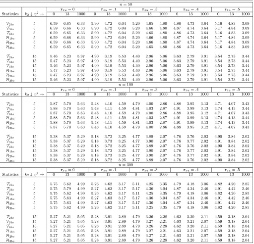
Table 2 reports the results. As before, rzu = 0 corresponds to exogenous instruments whilerzu6= 0 characterize invalid instruments. Also,η2≤613 is for weak identification and
η2 > 613 characterize strong identification. We see that all tests have an overall correct
level whether identification is strong or weak. In addition, level is controlled even for a
relatively small sample (n = 50) and moderate instrument endogeneity (rzu = 0.5). The maximal size distortion of the bootstrap tests is around 6.7% and is obtained whenn= 50
andk= 5,further with exogenous instruments (rzu= 0). This is a substantial improvement compared to standard DWH tests whose maximal rejection was as great as 100% [see Table
1]. Furthermore, it is interesting to note that when model parameters are completely non
identified (η2 = 0) or close so, all bootstrap tests have correct level irrespective of the size
of instrument endogeneity. However, the tests tend to be conservative when instruments
endogeneity is large and identification strong. This is mainly justified by the fact that
the effect of instrument endogeneity on the tests increases with identification strength (see
Theorems3.1-3.1and simulations in Table 1). When identification is strong and instrument
endogeneity is large, the quantiles of the null distribution of the statistics tend to explode,
as discussed in Theorem3.2. However, the non centrality parameter is always bounded with
probability when identification is weak, even if instrument endogeneity is large (Theorem
3.2). Therefore, the occurrence of the events [Wr <Qˆ∗(α)] is higher when identification is weak than when it is strong. This is particularly why the tests have correct level in all
Table 2. Rejection frequencies (in %) of bootstrap DWH-tests at nominal level 5%;n= 50; 100; 300
n= 50
rzu= 0 rzu=.1 rzu=.3 rzu=.4 rzu=.5
Statistics k2↓ η2→ 0 13 1000 0 13 1000 0 13 1000 0 13 1000 0 13 1000
T2bs 5 6.59 6.65 6.33 5.90 4.72 6.04 5.20 4.65 4.80 4.86 4.73 3.64 5.16 4.83 3.09
T3bs 5 6.59 6.66 6.33 5.90 4.72 6.04 5.20 4.66 4.80 4.87 4.74 3.64 5.17 4.84 3.09
T4bs 5 6.59 6.65 6.33 5.90 4.72 6.04 5.20 4.65 4.80 4.86 4.73 3.64 5.16 4.83 3.09
H1bs 5 6.59 6.66 6.33 5.90 4.72 6.04 5.20 4.66 4.80 4.87 4.74 3.64 5.17 4.84 3.09
H2bs 5 6.59 6.66 6.33 5.90 4.72 6.04 5.20 4.66 4.80 4.87 4.74 3.64 5.17 4.84 3.09
H3bs 5 6.59 6.65 6.33 5.90 4.72 6.04 5.20 4.65 4.80 4.86 4.73 3.64 5.16 4.83 3.09
T2bs 15 5.46 5.23 5.97 4.90 3.19 5.53 4.40 2.96 5.06 3.63 2.79 3.91 3.54 2.73 3.44
T3bs 15 5.47 5.23 5.97 4.90 3.19 5.53 4.40 2.96 5.06 3.63 2.79 3.91 3.54 2.73 3.44
T4bs 15 5.46 5.23 5.97 4.90 3.19 5.53 4.40 2.96 5.06 3.63 2.79 3.91 3.54 2.73 3.44
H1bs 15 5.47 5.23 5.97 4.90 3.19 5.53 4.40 2.96 5.06 3.63 2.79 3.91 3.54 2.73 3.44
H2bs 15 5.47 5.23 5.97 4.90 3.19 5.53 4.40 2.96 5.06 3.63 2.79 3.91 3.54 2.73 3.44
H3bs 15 5.46 5.23 5.97 4.90 3.19 5.53 4.40 2.96 5.06 3.63 2.79 3.91 3.54 2.73 3.44
n= 100
rzu= 0 rzu=.1 rzu=.3 rzu=.4 rzu=.5
Statistics k2↓ η2→ 0 13 1000 0 13 1000 0 13 1000 0 13 1000 0 13 1000
T2bs 5 5.87 5.70 5.63 5.48 4.10 4.59 4.79 4.00 2.86 4.88 3.95 3.12 4.71 4.07 3.43
T3bs 5 5.88 5.70 5.63 5.48 4.11 4.59 4.81 4.03 2.87 4.91 3.99 3.13 4.74 4.13 3.44
T4bs 5 5.87 5.70 5.63 5.48 4.10 4.59 4.79 4.00 2.86 4.88 3.95 3.12 4.71 4.07 3.43
H1bs 5 5.88 5.70 5.63 5.48 4.11 4.59 4.81 4.03 2.87 4.91 3.99 3.13 4.74 4.13 3.44
H2bs 5 5.88 5.70 5.63 5.48 4.11 4.59 4.81 4.03 2.87 4.91 3.99 3.13 4.74 4.13 3.44
H3bs 5 5.87 5.70 5.63 5.48 4.10 4.59 4.79 4.00 2.86 4.88 3.95 3.12 4.71 4.07 3.43
T2bs 15 5.38 5.37 5.29 5.18 3.72 3.25 4.77 3.89 2.07 4.76 3.76 2.02 4.90 3.84 2.02
T3bs 15 5.38 5.37 5.29 5.18 3.73 3.25 4.77 3.90 2.07 4.76 3.77 2.02 4.91 3.84 2.02
T4bs 15 5.38 5.37 5.29 5.18 3.72 3.25 4.77 3.89 2.07 4.76 3.76 2.02 4.90 3.84 2.02
H1bs 15 5.38 5.37 5.29 5.18 3.73 3.25 4.77 3.90 2.07 4.76 3.77 2.02 4.91 3.84 2.02
H2bs 15 5.38 5.37 5.29 5.18 3.73 3.25 4.77 3.90 2.07 4.76 3.77 2.02 4.91 3.84 2.02
H3bs 15 5.38 5.37 5.29 5.18 3.72 3.25 4.77 3.89 2.07 4.76 3.76 2.02 4.90 3.84 2.02
n= 300
rzu= 0 rzu=.1 rzu=.3 rzu=.4 rzu=.5
Statistics k2↓ η2→ 0 13 1000 0 13 1000 0 13 1000 0 13 1000 0 13 1000
T2bs 5 5.75 5.62 4.99 5.26 4.62 3.17 5.11 4.25 3.35 4.79 4.18 3.06 4.82 4.20 2.85
T3bs 5 5.75 5.79 4.99 5.27 4.63 3.17 5.17 4.36 3.04 4.87 4.34 2.46 4.91 4.42 2.46
T4bs 5 5.75 5.62 4.99 5.26 4.62 3.17 5.11 4.25 3.35 4.79 4.18 3.06 4.82 4.20 2.85
H1bs 5 5.75 5.63 4.99 5.27 4.63 3.17 5.17 4.36 3.04 4.87 4.34 2.46 4.91 4.42 2.46
H2bs 5 5.75 5.63 4.99 5.27 4.63 3.17 5.17 4.36 3.04 4.87 4.34 2.46 4.91 4.42 2.46
H3bs 5 5.75 5.62 4.99 5.26 4.62 3.17 5.11 3.25 3.35 4.79 4.18 3.06 4.82 4.20 2.85
T2bs 15 5.27 5.21 5.05 5.28 3.91 2.89 4.79 3.26 2.28 4.62 3.20 2.11 4.59 3.18 2.04
T3bs 15 5.27 5.21 5.05 5.28 3.91 2.89 4.79 3.27 2.21 4.63 3.21 2.07 4.59 3.18 2.04
T4bs 15 5.27 5.21 5.05 5.28 3.91 2.89 4.79 3.26 2.28 4.62 3.20 2.11 4.59 3.18 2.04
H1bs 15 5.27 5.21 5.05 5.28 3.91 2.89 4.79 3.27 2.21 4.63 3.21 2.07 4.59 3.18 2.04
H2bs 15 5.27 5.21 5.05 5.28 3.91 2.89 4.79 3.27 2.21 4.63 3.21 2.07 4.59 3.18 2.04
H3bs 15 5.27 5.21 5.05 5.28 3.91 2.89 4.79 3.26 2.28 4.62 3.20 2.11 4.59 3.18 2.04
5.
Empirical illustration
We illustrate our theoretical results through the trade and growth model [Frankel and
Romer (1999), Harrison (1996), Mankiw, Romer and Weil (1992)]. The model studies
the relationship between standards of living and openness. Because the trade share (ratio
of imports or exports to GDP) commonly used as an indicator of openness is possibly
endogenous, Frankel and Romer (1999) suggest instrumental variables method to estimate
the income-trade relationship. The basic structural equation studied is given by:
ln(wi) =β0+βTradei+γ1ln(Popi) +γ2ln(Areai) +ui, i= 1, . . . , n (5.1) wherewis the income per capita, Pop is the population and Area is country area. The
in-strumentZsuggested by Frankel and Romer (1999) is constructed on the basis of geographic
characteristics and the first stage specification is
Tradei=b0+b1Zi+c1ln(Popi) +c2ln(Areai) +Vi, i= 1, . . . , n. (5.2)
Concern has raised in recent studies that the instrument constructed in this way may be
invalid, weak, or both [see the review of Samuel and Michael (2009)].
Here, we want to assess the exogeneity of “Trade” taking into account a possibility
that Z may be invalid or weak. The data are from Frankel and Romer (1999) and contain
initially 150 countries for year 1985. The first stage F-statistic4 in ( 5.2) is about 13,
hence the constructed instrument is not very poor compared to Staiger and Stock (1997)’s
rule of thumb of 10. We use both the standard and bootstrap DWH tests to assess the
exogeneity of “Trade” ˙First, we observe that the OLS and 2SLS estimates ofβare 0.2809 and
2.0251 respectively, while the magnitude of the regression endogeneity parameter estimate
seems relatively small (ˆb = 0.0079) but is significantly different from zero at level 5%
(tˆb = 2.026 > 1.96). This corresponds to error-instrument covariance estimate of about
ˆ
σZu = 12.309 and the estimate of the covariance between structural and reduced-form errors (here Trade endogeneity parameter) of approximately ˆσZu=−0.0149.This suggests that the instrumentZ is not strictly exogenous. Hence, it is very likely that the discrepancy
4
between OLS and 2SLS estimates is more due to instrument endogeneity rather than trade
share exogeneity.
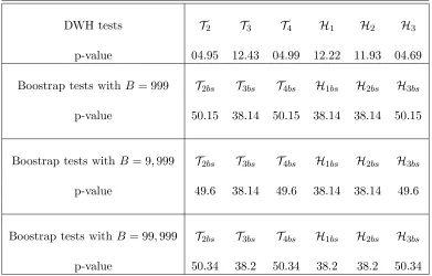
Table 3 presents the outcomes for both standard and boostrap tests. The bootstrap tests
are run for 999, 9,999 and 99,999 replications. The results indicate thatT2,T4andH3reject
the the exogeneity of the trade share at level 5%, butT3,H1 andH2 fail to reject it even at
level 10%, despite the large discrepancy between OLS and 2SLS estimates. The maximal
p-value is 12.43% and is obtained with T3. Since model identification is weak, it is more
likely that this contradiction among the DWH tests is attributable to instrument invalidity.
This is confirmed by the bootstrap tests (that account for instrument endogeneity) which
find no evidence against the exogeneity of trade share with p-values above 38%, even for
large bootstrap samples. This underscores how the standard DWH tests may be misleading
[image:23.595.111.502.399.649.2]if the instruments violate (even locally) the strict exogeneity assumption.
Table 3. Exogeneity of Trade in growth model (p-values in %)
DWH tests T2 T3 T4 H1 H2 H3
p-value 04.95 12.43 04.99 12.22 11.93 04.69
Boostrap tests with B = 999 T2bs T3bs T4bs H1bs H2bs H3bs p-value 50.15 38.14 50.15 38.14 38.14 50.15
Boostrap tests withB = 9,999 T2bs T3bs T4bs H1bs H2bs H3bs p-value 49.6 38.14 49.6 38.14 38.14 49.6
Boostrap tests with B= 99,999 T2bs T3bs T4bs H1bs H2bs H3bs p-value 50.34 38.2 50.34 38.2 38.2 50.34
6.
Conclusion
This paper focuses on linear structural models and investigate the size of the standard
Durbin-Wu-Hausman tests for exogeneity when instruments violate “strict exogeneity”.
which clearly show that these tests are severely size distorted even for a small correlation
between instruments and the structural error. A Monte carlo experiment suggests that the
maximal size distortion can be as great as 100% when instrument endogeneity is fixed and
identification strong.
We then propose a bootstrap procedure to correct the size of the tests. The simulations
indicate that the bootstrap tests have an overall good performance even for moderate
in-strument endogeneity. We apply our theoretical framework to the trade and growth model
of Frankel and Romer (1999). We find that the instrument constructed on the basis of
countries geographic characteristics is not strictly exogenous. Therefore, the use of the
standard DWH tests for assessing the exogeneity of the trade variable lead to conflicting
results, though the structural parameter is identified [see Dufour and Taamouti (2007)].
More precisely, the tests T2, T4 and H3 find evidence against the exogeneity of the trade
variable with ap-values less than 5%, whileT3,H1andH2 cannot reject the exogeneity even
at level 10%. However, all proposed bootstrap tests that account for instrument
endogene-ity conclude the non rejection of exogeneendogene-ity with p-values above 38%. This suggests that
the large discrepancy between OLS and 2SLS estimates is more attributable to instrument
APPENDIX
A.
Proofs
Lemma A.1 Suppose Assumptions2.1-2.2 are satisfied and rank(Π) =m. If συu= 0, then:
(i) βˆ→p β, ˜β→p β, β˜−βˆ→p 0;
(ii) √n(ˆβ−β) →d N(Π′QZΠ+ΣV)−1Π′d, σ2u(Π′QZΠ+ΣV)−1,
√
n(˜β−β) →d N(Π′QZΠ)−1Π′d, σ2u(Π′QZΠ)−1,
√
n(˜β−βˆ) →d N τd, σ2u[(Π′QZΠ)−1−(Π′QZΠ+ΣV)−1] whereτd= [(Π′QZΠ)−1−(Π′QZΠ+ΣV)−1]Π′d.
Proof of Lemma A.1 First, observe that ˆβ−β˜ as:
ˆ
β−β = ΩˆLS−1X′u/n, β˜−β = ˆΩ−1
IVX′PZu/n,
˜
β−βˆ = ΩˆIV−1X′PZu/n−ΩˆLS−1X′u/n. (A.1)
If Assumptions2.1-2.2hold and if further rank(Π) =mandσυu= 0, then ˆΩLS p
→Π′QZΠ+ΣV,
ˆ ΩIV
p
→ Π′QZΠ, X′u/n = Π′Z′u/n+V′u/n p
→ 0, and X′P
Zu/n = Π′Z′u/n+V′PZu/n p
→ 0.
Thus LemmaA.1-(i) holds.
Now from (A.1), we have: √n(ˆβ −β) = ˆΩLS−1X′u/√n, √n(˜β −β) = ˆΩ−1
IVX′PZu/√n, and
√
n(˜β−βˆ) = ˆΩIV−1X′P
Zu/√n−ΩˆLS−1X′u/
√
n. Under the condition of the lemma, we haveX′u/√n=
Π′√1nPni=1Ziui+√1nPni=1(Viui−σV u) d
→Π′(ψzu+d) +ψV u, and X′PZu/√n=Π′Z′u/√n+
V′P
Zu/√n=Π′Z′u/√n+op(1) d
→Π′(ψzu+d). So, we find
√
n(ˆβ−β) →d (Π′QZΠ+ΣV)−1[Π′(ψzu+d) +ψV u],
√
n(˜β−β)→d (Π′QZΠ)−1Π′(ψzu+d)
√
n(˜β−βˆ) →d Ψd= (Π′QZΠ)−1Π′(ψzu+d)−(Π′QZΠ+ΣV)−1[Π′(ψzu+d) +ψV u].
Under H0 and Assumption 2.2, we have (ψzu+d, ψV u) ∼N
d, σ2u
QZ 0
0 ΣV
jointly, so
that LemmaA.1-(ii) follows directly.
(i) ˆβ→p β, β˜−β→d R
Rk×mN νd, σ
2
u[(Π0+Q−Z1x2)′QZ(Π0+Q−Z1x2)]−1pdf(x2)dx2;
(ii) β˜−βˆ→d R
Rk×mN νd, σ
2
u[(Π0+Q−Z1x2)′QZ(Π0+Q−Z1x2)]−1pdf(x2)dx2
whereνd≡νd(x2) = [(Π0+Q−Z1x2)′QZ(Π0+Q−Z1x2)]−1(Π0+QZ−1x2)′d andpdf(.)is the probability density function of ψzv.
Proof of Lemma A.2 Let Π = Π0/√n where Π0 is a k ×m constant matrix. When
συu = 0, we have ˆΩLS p
→ ΣV > 0 and X′u/n p
→ 0 so that ˆβ −β = op(1) and ˜β −βˆ =
(nΩˆIV)−1X′PZu−ΩˆLS−1X′u/n = (nΩˆIV)−1X′PZu+ 0p(1) = ˜β − β + op(1). Since nΩˆIV =
X′P
ZX = (X′Z/√n)(Z′Z/n)−1(Z′X/√n) and Z′Z/n p
→ QZ, Z′X/√n d
→ QZΠ0+ψzv, it is
clear that nΩˆIV d
→ (Π0+Q−Z1ψzv)′QZ(Π0+Q−Z1ψzv). By the same way, we have X′PZu d
→
(Π0+Q−Z1ψzv)′(ψzu+d). Therefore ˆβ−β˜= ˜β−β+op(1) d
→ΨZv,d where
ΨZv,d = [(Π0+QZ−1ψzv)′QZ(Π0+QZ−1ψzv)]−1(Π0+QZ−1ψzv)′(ψzu+d).
Because ψzv is independent of ψzu under H0, we have ΨZv,d|ψzv ∼
N νd, σ2u[(Π0+Q−Z1ψzv)′QZ(Π0+Q−Z1ψzv)]−1
, where νd = [(Π0 + QZ−1ψzv)′QZ(Π0 +
Q−Z1ψzv)]−1(Π0+Q−Z1ψzv)′d. By integrating with respect toψzv, the result follows.
Proof of Theorem3.1 Let rank(Π) =m and suppose Assumptions2.1-2.2 hold withσυu= 0.
From LemmaA.1, we have
ˆ
σ2 = u′u/n−(u′X/n) ˆΩ−LS1(X′u/n)→p σ2u, σ˜22= ˆσ2+ 0p(1) p
→σ2u (A.2)
˜
σ2 = u′u/n−2(u′X/n) ˆΩIV−1(X′PZu/n) + (u′PZX/n) ˆΩIV−1(X′PZu/n) p
→σ2u. (A.3)
LemmaA.1 along with (A.2)-(A.3) then entail that
T2 d
→ mσ12 u
Ψd′[(Π′QZΠ)−1−(Π′QZΠ+ΣV)−1]−1Ψd∼
1 mχ
2(m;µ
d),
Tl,Hj →d 1
mΨ ′
d[(Π′QZΠ)−1−(Π′QZΠ+ΣV)−1]−1Ψd∼χ2(m;µd), , l= 3,4 and j = 1,2,3
where µd= σ12uτ′d[(Π′QZΠ)−1−(Π′QZΠ+ΣV)−1]−1τd=k¯τdk2, ¯τd= σ1
u[(Π
′QZΠ+ΣV)−1−
(Π′QZΠ)−1]−1/2τd= σ1
u[(Π
′QZΠ)−1−(Π′QZΠ+ΣV)−1]1/2Π′d.
Proof of Theorem3.2 As in the above proof of Theorem3.1, we still have:
ˆ
σ2 = u′u/n−(u′X/n) ˆΩ−LS1(X′u/n)→p σ2u, σ˜22= ˆσ2+ 0p(1) p
However, we can see from LemmaA.2that we now have
˜
σ2 = u′u/n−2(u′X/n) ˆΩ−1
IV(X′PZu/n) + (u′PZX/√n)(nΩˆIV)−1(X′PZu/√n) d
→ σ¯2u=σ2u+ΨZv,′ d(Π0+Q−Z1ψzv)′QZ(Π0+Q−Z1ψzv)ΨZv,d≥σ2u. (A.5)
The independence between ψzu and ψzv under H0, along with Lemma A.2 then imply that
Ψ′
Zv,d(Π0+Q−Z1ψzv)′QZ(Π0+Q−Z1ψzv)ΨZv,d|ψzv ∼σ2uχ2(m;kν¯dk2). Therefore, ˜σ2|ψzv d
→σ2 u[1 +
χ2(m;k¯ν
dk2)]≥σ2u, where ¯νd= 1
σu[(Π0+Q −1
Z ψzv)′QZ(Π0+Q−Z1ψzv)]−1/2(Π0+QZ−1ψzv)′d. By
the same way, we get T2|ψzv
d
→ 1 mχ
2(m;k¯ν
dk2), T4,H3|ψzv d
→ χ2(m;kν¯
dk2), and T3,Hj|ψzv d
→
χ2(m;kνd¯ k2)
1+χ2(m;k¯νdk2 ≤χ
2(m; k¯ν
References
Anderson, T. W., Rubin, H., 1949. Estimation of the parameters of a single equation in a complete
system of stochastic equations. Annals of Mathematical Statistics 20, 46–63.
Ashley, R. , 2009. Assessing the credibilility of instrumental variables inference with imperfect
in-struments via sensitivity analysis. Journal of Applied Econometrics 24(2), 325–337.
Berkowitz, D., Caner, M. , Fang, Y. , 2008. Are nearly exogenous instruments reliable?. Economics
Letters 101, 20–23.
Bound, J., Jaeger, D. A. , Baker, R. M. , 1995. Problems with instrumental variables estimation
when the correlation between the instruments and the endogenous explanatory variable is weak.
Journal of the American Statistical Association 90, 443–450.
Chaudhuri, S. , Rose, E. , 2009. Estimating the veteran effect with endogenous schooling when
instruments are potentially weak. Technical report, IZA Discussion Papers No. 4203.
Choi, I., Phillips, P. C. B., 1992. Asymptotic and finite sample distribution theory for IV estimators
and tests in partially identified structural equations. Journal of Econometrics 51, 113–150.
Davidson, R. , Mackinnon, J. G. , 2007. Testing for consistency using artificial regressions.
Compu-tational Statistics and Data Analysis 50, 3259–3281.
Doko Tchatoka, F. , 2011. Subset hypotheses testing and instrument exclusion in the linear IV
regression. Technical report, School of Economics and Finance, University of Tasmania Hobart,
Australia.
Doko Tchatoka, F. , Dufour, J.-M. , 2008. Instrument endogeneity and identification-robust tests:
some analytical results. Journal of Statistical Planning and Inference 138(9), 2649–2661.
Doko Tchatoka, F., Dufour, J.-M., 2011a. Exogeneity tests and estimation in IV regressions.
Tech-nical report, Department of Economics, McGill University, Canada Montr´eal, Canada.
Doko Tchatoka, F., Dufour, J.-M., 2011b. On the finite-sample theory of exogeneity tests with
pos-sibly non-gaussian errors and weak identification. Technical report, Department of Economics,
McGill University, Canada Montr´eal, Canada.
Dufour, J.-M., Taamouti, M., 2007. Further results on projection-based inference in IV regressions
with weak, collinear or missing instruments. Journal of Econometrics 139(1), 133–153.
Durbin, J., 1954. Errors in variables. Review of the International Statistical Institute 22, 23–32.
Frankel, J. A., Romer, D., 1999. Does trade cause growth?. American Economic Review 89(3), 379–
Guggenberger, P. , 2010. The impact of a Hausman pretest on the size of the hypothesis tests.
Econometric Theory 156, 337–343.
Guggenberger, P., 2011. On the asymptotic size distortion of tests when instruments locally violate
the exogeneity assumption. Econometric Theory forthcoming.
Hall, A. R., Rudebusch, G. D., Wilcox, D. W., 1996. Judging instrument relevance in instrumental
variables estimation. International Economic Review 37, 283–298.
Hansen, C., Hausman, J., Newey, W., 2008. Estimation with many instrumental variables. Journal
of Business and Economic Statistics 26(4), 398–422.
Harrison, A., 1996. Oponness and growth: a time-series, cross-country analysis for developing
coun-tries. Journal of Development Economics 48, 419–447.
Hausman, J., 1978. Specification tests in econometrics. Econometrica 46, 1251–1272.
Hausman, J. , Hahn, J. , 2005. Estimation with valid and invalid instruments. Annales d’´Economie
et de Statistique 79–80, 25–57.
Imbens, G. W., 2003. Sensitivity to exogeneity assumptions in program evaluation. American
Eco-nomic Review 93(2), 126–132.
Imbens, G. W., Koles´ar, M., Chetty, R., Friedman, J., Glaeser, E., 20011. Inference and identification
with many invalid instruments. Technical report, Department of Economics, Havard University
Boston, MA.
Kiviet, J. F., Niemczyk, J., 2006. On the limiting and empirical distribution of IV estimators when
some of the instruments are invalid. Technical report, Department of Quantitative Economics,
University of Amsterdam Amsterdam, The Netherlands.
Kleibergen, F., 2005. Testing parameters in GMM without assuming that they are identified.
Econo-metrica 73, 1103–1124.
Mankiw, N. G., Romer, D. , Weil, D. N. , 1992. A contribution to the empirics of economic growth.
The Quarterly Journal of Economics 107(2), 407–437.
Moreira, M. J. , 2003. A conditional likelihood ratio test for structural models. Econometrica
71(4), 1027–1048.
Murray, P. M., 2006. Avoiding invalid instruments and coping with weak instruments. The Journal
of Economic Perspectives 20(4), 111–132.
Samuel, B., Michael, A. C., 2009. Blunt instruments: A cautionary note on establishing the causes
Sargan, J., 1958. The estimation of economic relationships using instrumental variables.
Economet-rica 26(3), 393–415.
Shea, J., 1997. Instrument relevance in multilinear models: A simple measure. Review of Economics
and Statistics 79, 348–352.
Staiger, D., Stock, J. H., 1997. Instrumental variables regression with weak instruments.
Economet-rica 65(3), 557–586.
Stock, J. H. , Yogo, M. , 2005. Testing for weak instruments in linear IV regression. In: D. W.
Andrews , J. H. Stock, eds, Identification and Inference for Econometric Models: Essays in
Honor of Thomas Rothenberg . Cambridge University Press, Cambridge, U.K. , chapter 6 ,
pp. 80–108.
Wu, D.-M., 1973. Alternative tests of independence between stochastic regressors and disturbances.
Econometrica 41, 733–750.
Wu, D.-M., 1974. Alternative tests of independence between stochastic regressors and disturbances: