The Effect of Pension on the Optimized
Life Expectancy and Lifetime Utility
Level
Shin, Inyong
September 2012
Online at
https://mpra.ub.uni-muenchen.de/41374/
and Lifetime Utility Level
Inyong Shin∗
Abstract
In this paper, we analyze the effect of a pension system on the life expectancy and the
lifetime utility level using a cross country data and an optimal dynamic problem of individuals
who live in continuous and finite time. From the data, we find that 1) Happiness can be almost
explained by income per capita. 2) Depending on income per capita, the pension system can
make life span longer or shorter and can raise or reduce the level of happiness. Our model
yields some results which are consistent with the results from the data: i) Life expectancy is
not always proportional to lifetime utility. ii) The pension system can make life expectancy
longer or shorter. This paper suggests that it is not always true that the pension system
improves the lifetime utility level.
JEL Classification Codes: C61, H55, I31
Keywords: pension system, optimized life expectancy, lifetime utility level, health investments
∗Department of Economics, Asia University,
5-24-10 Sakai Musashino Tokyo 180-8629 Japan, Tel.: +81-422-36-5259,
Fax: +81-422-36-4042,
e-mail addredss: [email protected]
1
Introduction
According to an anecdote in Europe, as soon as a pension system was introduced, the number of
people who jog in the park for their health increased. Believe it or not, under the pension system,
it looks like a good deal, if we live long enough. This paper analyzes the effect of a pension system
on the life expectancy and the lifetime utility level. There are many literatures on the effect of
rising longevity on some economic variables as saving rate, growth rate, labor market, education,
etc. For example, Bloom et al. (2007) and Dushi et al. (2010), Lee et al. (2000) etc. examine
the effects of improvements in health or life expectancy on social security system and saving rate.
Weil (2007), Acemoglu and Johnson (2007), Zhang and Zhang (2004), Zhang et al. (2001), etc.
analyze the effects of improvements in health or life expectancy on economic growth. Zhang et al.
(2003) shows that rising longevity encourages both savings and earlier retirement. Gorski et al.
(2007) studies the effects of a pension reform on the educational level of the economy. Pecchenino
and Utendorf (1999), de la Croix and Licandro (1999), Cipriani (2000), Boucekkine, et al. (2002,
2003), Pecchenino and Pollard (1997, 2002) etc. analyze the effect of longer life span on economic
growth through the level of schooling and human capital accumulation. Recently, Pestieau and
Ponthiere (2012) surveys the various contributions to the impact of changes in longevity on various
public policies. However, there is little research on the opposite direction, that is, the economic
variables, except the level of income, affect life expectancy or health. This paper is different from
previous researches in that a pension system is the cause, and the life expectancy and the lifetime
utility level are its effects.
A vast amount of empirical and theoretical researches about the economic welfare of a pension
system has been accumulated. The main results of some previous studies on pension system
and economic welfare can be summarized as follows: under a fully funded system, the economic
welfare is not affected, however, under a pay-as-you-go pension system, depending on the economic
situations and generations, the economic welfare might be both improved or worsened. The
public pension system as a risk-hedging device can increase welfare by providing a certainty in
the imperfect market. (Shiller, 1999, Krueger and Kubler, 2002, Marcos and
S´anchez-Martin, 2006, Bohn, 2009, etc.) The compulsory pension system which is one of the forced saving
policies can lead to high saving rates. Meanwhile, the public pension system crowds out the
private savings. It can have a negative effect on the capital accumulation and can retard growth.
overall welfare impact depends on the balance between the insurance effect and the crowding-out
effect. In this paper, we show that the pension system has both positive and negative effect on
welfare using a cross country data. More specifically, the pension system has a positive effect on
welfare when income per capita is low, but the pension system has a negative effect on welfare
when income per capita is high.
We compare the utility level under the restriction of the pension system as a compulsory saving
with the utility level without the restriction. Many previous researches analyze economic welfare
using overlapping generation models. We use the optimal dynamic problem of individuals who live
in continuous time, but not discrete time which is used in the overlapping generation models. (e.g.
Chakraborty, 2004, S´anchez-Marcos and S´anchez-Martin, 2006, Ponthiere, 2009, etc.) This is one
of the differences of our model from the previous models. To tell more specifics, in many previous
overlapping generation models, the maximum life span is given (e.g., two-period or three-period)
and the survival probability is introduced and the life expectancy is calculated by the average
of the longevity of the people who live to the maximum life span and the people who die before
the maximum life span depending on the the survival probability. Actually, in two-period model,
only two kinds of ages (i.e, one-period-old and two-period-old) exist and nobody survives more
than the given period even thougn the life expectancy has variations. However, our model is
handled under continuous time and the agents decide the terminal point of the continuous model
for oneself to maximize his/her life time utility. Like lifetime uncertainty models, e.g., Pecchenino
and Pollard (1997), Chakraborty (2004), Momota, et al (2005), etc., we assume that it is possible
to extend life span by the effort of an individual through health investments.1 For example, eating
good food, taking some nutritional supplements, getting in shape by going to the gym, investing
in the development of medical technology, etc., longevity will arise due to the given examples
on health investments. In reality, it is well known that coronary heart disease (CHD) mortality
is highly influenced by the major risk factors, e.g., serum cholesterol, systolic blood pressure,
diabetes, smoking habits, high alcohol consumption, lack of exercise and stress, etc. Lifestyle
changes through individual’s efforts (e.g., healthier diet, physical exercise, cessation of smoking
and drinking) and medications have been shown to be effective in reducing coronary disease. If
we can eliminate the risk factors, the life expectacny will undoubtedly grow.
An individual distributes his/her budget to his/her basic needs and to his/her health
invest-1Lifetime uncertainty models assume that the health investments can increase the surviving probability. However,
ments to maximize his/her lifetime utility. We consider that the individual’s longevity is based
from the result of the individual’s utility maximization problem. This means that the
individ-ual’s longevity is an endogenous variable and not exdogenous variable. We investigate how the
optimized life span and the lifetime utility level can be changed by a pension system.
In Section 2, using a cross country data, we show the following: 1) Income per capita can
almost explain happiness. The positive correlationship between life expectancy and happiness is
a spurious relationship in which two variables have no direct causal connection. In reality, income
per capita which is an unseen variable has caused both. And the life span does not have much
influence on happiness. 2) Depending on income per capita, the pension system can make life
span longer or shorter. 3) Depending on income per capita, the pension system can raise or reduce
the level of happiness.In Section 3, our model yields two important results: i) Life expectancy is
not always proportional to lifetime utility level. ii) Pension system can make the life span longer
or shorter. The life span depends on the type of pension system. From the combination of the
results i) and ii), it is possible that A) the pension system makes the life span longer and increases
the utility level. B) the pension system makes the life span longer, however decreases the utility
level. C) the pension system makes the life span shorter and decreases the utility level. Case 1 is
preferable. But Case 2 and 3 are not preferable cases, but could possibly happen. Our results A),
B) and C) from the optimal problem are consistent with 2) and 3) that we will see in the data in
Section 2.
This paper is organized as follows: In Section 2, we confirm the relationship among income
per capita, the presence or absence of a pension system, happiness and life expectancy using a
cross country data. Section 3 presents the model and drives the benchmark outcomes. In section
4, we introduce the pension system to the benchmark. Section 5 solves the models numerically
and analyzes the results and concludes. And finally, we include an Appendix.
2
Empirical Facts
2.1 Data
We take up income per capita, life expectancy and the presence or absence of a pension system
as the determinants of happiness. The three variables are thought to be the variable that look at
an economic side, a biological side and a social systematic side to decide the level of happiness,
used by this paper can be easily acquired on the internet. The happiness index and the life
expectancy are available from World Database of Happiness and GDP per capita is also found
in Penn World table. The presence or absence of a pension system is obtained from Table 1 of
Bloom et al. (2007). World Database of Happiness releases the averages of the happiness index
and the life expectancy from 2000 to 2009 by country, respectively. The happiness index run from
0 to 10. GDP per capita uses the variable “rgdpch” in Penn World Table 7.1. According to the
Penn World Table 7.1, the definition of variable “rgdpch” is that PPP converted GDP per capita
(chain series), at 2005 constant prices. We calculate the average of GDP per capita from 2000
to 2009 to meet the happiness index and the life expectancy in World Database of Happiness.
We used the logarithm for GDP per capita, in the following analysis. The pension data which
are dummy variables for the presence or absence of a pension system show the situation in 2002.
The value is one when they have a pension system and the value is zero when they do not have a
pension system. The pension data use “Universal Coverage”.According to Bloom et al. (2007),
the definition is that the dummy variable of universal coverage indicates whether the system
covers all workers or not. Table 1 shows the detailed data source. World Database of Happiness,
Penn World Table 7.1 and the pension data in 2002 of Bloom et al. (2007) listed 149, 190 and
61 countries, respectively. We focus on the 61 countries which are included in all the three data
sets. Table A1 in Appendix contains the basic information of the 61 countries.
5 6 7 8 9 10 11
2
4
6
8
5 6 7 8 9 10 11
2
4
6
8
(1) Income and Happiness
Income per capita
Happiness
x: P=0 o: P=1
20 30 40 50 60 70 80 90
2
4
6
8
20 30 40 50 60 70 80 90
2
4
6
8
(2) Life Expectancy and Happiness
Life expectancy
Happiness
x: P=0 o: P=1
0 1
2
4
6
8
0 1
2
4
6
8
(3) Pension system and Happiness
The presence or absence of a pension system
Happiness
[image:6.595.75.521.485.711.2]x: P=0 o: P=1
Figure 1: Income, life expectancy, pension system and happiness
Table 1: Data sources
Indicators Database URL
Satisfaction
with life
(Happiness)
World Database of Happiness
http://worlddatabaseofhappiness.eur.nl/
Life
ex-pectancy
World Database of Happiness
http://worlddatabaseofhappiness.eur.nl/
Life
ex-pectancy at birth, total (years)
World Bank http://data.worldbank.org/indicator/SP.DYN.LE00.IN
Happy life
years∗
World Database of Happiness
http://worlddatabaseofhappiness.eur.nl/
Per capita
GDP
Penn World
Table
https://pwt.sas.upenn.edu/
*) Happy life years are calculated by the product of Satisfaction with life and Life expectancy.
absence of a pension system and happiness. In Figure (1), each vertical axis shows the happiness.
o’s and +’s represent the countries that have the pension system and do not, respectively. It
appears that there are positive relationships between income per capita and happiness, between
life expectancy and happiness, between pension and happiness, respectively. The coefficients of
correlation are r(income per capita,happiness) = 0.833,r(life expectancy,happiness) = 0.788,
r(pension,happiness) = 0.390.
2.2 Regression Analysis
2.2.1 Happiness
We investigate the relationships between happiness and income per capita, between happiness
and life expectancy, between happiness and pension system. The happiness is treated as the
dependent variable. We use linear regression models as Eq. (1) to (4).Eq. (1) has a single
regressor, income per capipa. Eq. (2) has two regressors, income per capita and life expectancy.
And, Eq. (3) and Eq. (4) have two regressors, income per capita and the presence or absence of
a pension system.We estimate the variables by the maximum likelihood esimation (MLE). The
variables. Hi,yi,Li andPi represent the happiness level, income per capita, life expectancy and
the presence or absence of a pension system in a country i, respectively. Let us assume that the
errors ϵi is identically distributed, independent random variables with ϵi ∼ N(0, σ2). Table 2 is
the estimation results of Eq. (1) to (4), respectively.
Hi =β0+β1yi+ϵi (1)
Hi =β0+β1yi+β2Li+ϵi (2)
Hi =β0+β1yi+β2Pi+ϵi (3)
[image:8.595.157.452.347.601.2]Hi = (1−Pi)(β0+β1yi) +Pi(γ0+γ1yi) +ϵi (4)
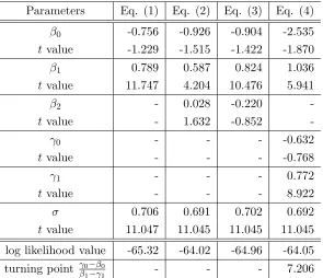
Table 2: Estimation results
Parameters Eq. (1) Eq. (2) Eq. (3) Eq. (4)
β0 -0.756 -0.926 -0.904 -2.535
t value -1.229 -1.515 -1.422 -1.870
β1 0.789 0.587 0.824 1.036
t value 11.747 4.204 10.476 5.941
β2 - 0.028 -0.220
-t value - 1.632 -0.852
-γ0 - - - -0.632
t value - - - -0.768
γ1 - - - 0.772
t value - - - 8.922
σ 0.706 0.691 0.702 0.692
t value 11.047 11.045 11.045 11.045
log likelihood value -65.32 -64.02 -64.96 -64.05 turning point γ0−β0
β1−γ1 - - - 7.206
The upper and lower show the estimated values andt values, respectively.
The estimated all β1’s for income per capita (y) in Eq. (1), (2) and (3) are positive and
significant, but the estimatedβ2’s in Eq. (2) and Eq. (3) for life expectancy (L) and the presence
or absence of a pension system (P) are not significant, respectively.We know that happiness can
be almost explained by income per capita and that the life expectancy and the pension system
contribute little to happiness. And we also know that from Eq. (4), the intercept (β0 < γ0)
and the slope (β1> γ1) of the line relating per capita income and happiness are statistically and
say that when income per capita is low, happiness is higher with the pension system than without
it, otherwise, when income per capita is high, happiness is higher without the pension system
than with it. The turning point is about income per capita 1,347 = exp(7.206) which is small
enough. When income level is low, the pension system make people happy. On the other hand,
when income level is high, the pension system which is a kind of the forced saving policies prevents
individuals from maximizing his/her utility. In other words, it suggests that to plan his/her own
future and to optimize his/her utility by himself/herself can be happier without the pension.
5 6 7 8 9 10 11
2
4
6
8
5 6 7 8 9 10 11
2
4
6
8
(1) Income and Happiness
Income per capita
Happiness Eq.(1) Eq.(4) P=0 Eq.(4) P=1 x: P=0 o: P=1
20 30 40 50 60 70 80 90
−2
−1
0
1
2
20 30 40 50 60 70 80 90
−2
−1
0
1
2
(2) Life expectandy and Happiness
Life expectancy
Residual of Happiness
x: P=0 o: P=1
−20 −10 0 10 20
−2
−1
0
1
2
−20 −10 0 10 20
−2
−1
0
1
2
(3) Life expectancy and Happiness
Residual of life expectancy
Residual of happiness
[image:9.595.81.521.236.458.2]x: P=0 o: P=1
Figure 2: Income, life expectancy and happiness
We visualize the regression results from Eq. (1) to Eq. (4) in Figure 2. Figure 2 (1) shows
regression lines based on Eq. (1) and Eq. (4). In comparison with the red line (P = 0) and the
blue line (P = 1), the slope of the red line is steeper than that of the blue line. We can find that
when income per capita is low, the blue line is upper than the red line, that is, happiness is higher
with the pension than without it, but when income per capita is high, the opposite occures. The
red line is upper than the blue line, that is, happiness is higher without the pension than with
it. We draw the black line that best fits the data point in Figure 2 (1) from Eq. (1), and then,
for each country, we measure the gap between the country’s actual level of happiness and the
level predicted by the fitted line. Figure 2 (2) shows the relationship between the residual part
of happiness and life expectancy. Because happiness is explained by income per capita, there
is not high corellatonship between the residuals and life expectancy. The correlation coefficient
relationship between the residuals of life expectancy of the independent variable income per capita
and the residuals of happiness of the independent variable income per capita. When we remove
the influence of income on life expectancy and happiness, the relationship between both variables
is not so strong (r=0.205). From the result of Figure 2 (2) and (3), we know that the positive
correlationship between life expectancy and happiness in Figure 1 (2) is a spurious relationship.
Even if we can see the relationship that the longer life expectancy looks happier, we know that
two variables have no direct causal connection and the income per capita actually works behind
the two variables, the life expectancy and happiness. The increasing life span without increasing
income does not necessarily increase happiness. It unfortunately suggests that the survival itself
is not always making utility high.
2.2.2 Life Expectancy and Happy Life Year
First, we investigate the relationships between the life expectancy and income per capita, between
the life expectancy and the pension system. The life expectancy is treated as the dependent
variable. We do regression analysis using Eq. (5) to Eq. (7). Eq. (5) has a single regressor,
income per capita. Eq. (6) and Eq. (7) have two regressors, income per capita and the presence
or absence of a pension system.We estimate the variables by the maximum likelihood esimation
like as what we did in Section 2.2.1.
Second, we also investigate the relationships between the happy life year and income per
capita, between the happy life year and the pension system. The happy life year is treated as the
dependent variable. The happy life years are calculated by the product of the level of happiness
and life expectancy. We do regression analysis using Eq. (8) to Eq. (10). HLi represents the
happy life year.
Li =β0+β1yi+ϵi (5)
Li =β0+β1yi+β2Pi+ϵi (6)
HLi=β0+β1yi+ϵi (8)
HLi=β0+β1yi+ +β2Pi+ϵi (9)
[image:11.595.110.501.212.471.2]HLi= (1−Pi)(β0+β1yi) +Pi(γ0+γ1yi) +ϵi (10)
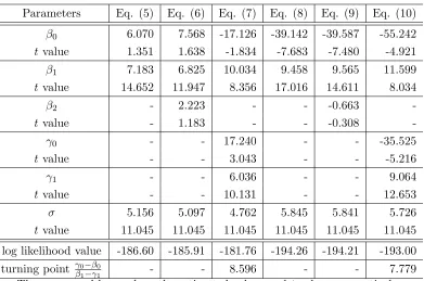
Table 3: Estimation results
Parameters Eq. (5) Eq. (6) Eq. (7) Eq. (8) Eq. (9) Eq. (10)
β0 6.070 7.568 -17.126 -39.142 -39.587 -55.242
t value 1.351 1.638 -1.834 -7.683 -7.480 -4.921
β1 7.183 6.825 10.034 9.458 9.565 11.599
t value 14.652 11.947 8.356 17.016 14.611 8.034
β2 - 2.223 - - -0.663
-t value - 1.183 - - -0.308
-γ0 - - 17.240 - - -35.525
t value - - 3.043 - - -5.216
γ1 - - 6.036 - - 9.064
t value - - 10.131 - - 12.653
σ 5.156 5.097 4.762 5.845 5.841 5.726
t value 11.045 11.045 11.045 11.045 11.045 11.045
log likelihood value -186.60 -185.91 -181.76 -194.26 -194.21 -193.00 turning point γ0−β0
β1−γ1 - - 8.596 - - 7.779
The upper and lower show the estimated values andt values, respectively.
Table 3 shows the estimation results by Eq. (5) to Eq. (10). The results in Table 3 are
very similar to the results obtained with happiness as an independent variable in Table 1. The
estimated all β1’s for income per capita (y) are positive and significant, but the estimated β2’s
for the presence or absence of a pension system (P) are not significant.From Eq. (6) and Eq.
(9), we know that because both the life expectancy and the happy life year are explained by
income per capita, the pension system itself has no explanatory power to both the life expectancy
and the happy life year. It means that the pension system itself cannot extend the life span and
the happy life year. From Eq. (7) and Eq. (10), we know that depending on the presence or
absence of a pension system, the intercept (β0< γ0) and the slope (β1> γ1) of the regression line
are statistically and significantly different. From the results, we can say that when income per
capita is low, the life expectancy and the happy life year are longer with the pension system than
without it, otherwise, when income per capita is high, the life expectancy and the happy life year
are about income per capita 5,410 = exp(8.596) and 2,390 = exp(7.779), respectively. Anyhow,
the values are low. In countries with low income levels, both the life expectancy and the happy
life year are increased by the pension system, on the other hand, in countries with high income
levels, both the life expectancy and the happy life year are decreased by the pension system. It
suggests that in countries with a high level of income, the individual’s utility optimizations are
being hampered by the savings forced by the pension system.
5 6 7 8 9 10 11
20
40
60
80
5 6 7 8 9 10 11
20
40
60
80
(1) Income and Life Expectancy
Income per capita
Lif
e e
xpectancy
Eq.(5) Eq.(7) P=0 Eq.(7) P=1
x: P=0 o: P=1
5 6 7 8 9 10 11
20
40
60
80
5 6 7 8 9 10 11
20
40
60
80
(2) Income and Happy Life Years
Income per capita
Happ
y lif
e y
ears
Eq.(8)
Eq.(10) P=0 Eq.(10) P=1
[image:12.595.158.441.217.437.2]x: P=0 o: P=1
Figure 3: Income, life expectancy and happiness
Figure 3 shows regresion lines. Figure 3 (1) shows the relationship between income per capita
and the life expectancy. Figure 3 (2) shows the relationship between income per capita and the
happy life year. When we compare the red lines (P = 0) and the bule lines (P = 1), Figure 3
shows that the regression lines without the pension system are steeper than those with it.
2.2.3 Nonparametric estimation
We loosen the assumption of linear relationship between variables which we used in Section 2.2.1
and Section 2.2.2. We estimate the relationship by a nonparametric estimation which estimates the
regression function without assuming any specific form. Eq. (11) to Eq. (14) are the unknown
regression equations. The dependent variables in Eq. (11) to Eq. (14) are happiness, the life
expectancy and the happy life years and happiness, respectively. Each equation from Eq. (11)
to Eq. (13) have one regressor, income per capita and Eq. (14) has two regressors, income per
Hi =f(yi) +ϵi (11)
Li =f(yi) +ϵi (12)
HLi =f(yi) +ϵi (13)
Hi =f(yi, Pi) +ϵi (14)
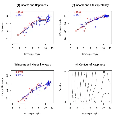
Figure 4 (1) to (4) are the regression results of Eq. (11) to Eq. (14), respectively. The
estimation results in Figure 4 (1) to (3) are not much different to the results obtained by assuming
a linear relationship like as what we did before. The red lines (P = 0) without the pension system
are steeper than the bule lines (P = 1) with the pension system. Because Eq. (14) has two
regressors, we depict the regression result by the contour line in Figure 4 (4). The contour line
shows the same level of happiness in the different combination of two variables which are income
per capital and pension system. When income per capita is low, it can be seen that the contour
lines are vertically-tilted. It means that regardless of whether the pension system is involved, the
level of happiness is almost the same. However, as income per capita increases, the contour lines
are no longer vertically-tilted. The contour lines begin to turn clockwise. For example, point A
where income per capita which is 8.5 without the pension system and point B where income per
capita which is 10.0 with the pension system have the same level of happiness, that is, the same
level of happiness is seven. In other words, if they have the same income, it is happier when there
is no pension system than when there is.
2.2.4 Check of Diminishing Marginal Increase of Life Expectancy
In countries with low income per capita, the increase of their life expectancy has a tendency to be
big, in contrast, in countries with high income per capita, the increase of their life expectancy has
a tendency to be small, that is, as income is increased, the marginal increase of the life expectancy
is apt to decrease. We check whether the diminishing phenomenon is the cause that the regression
lines in countries with low income per capita have steep slopes and the regression lines in countries
with high income per capita have glacis slopes, because it is possible that countries with high
income per capita tend to establish a pension system, in contrast, the countries with low income
per capita tend not to establish a pension system.
We do regression analysis using Eq. (15) and Eq. (16).2 We regress the change of life
5 6 7 8 9 10 11
2
4
6
8
5 6 7 8 9 10 11
2
4
6
8
(1) Income and Happiness
Income per capita
Happiness
x: P=0 o: P=1
5 6 7 8 9 10 11
20
40
60
80
5 6 7 8 9 10 11
20
40
60
80
(2) Income and Life expectancy
Income per capita
Lif
e e
xpectandy
x: P=0 o: P=1
5 6 7 8 9 10 11
20
40
60
80
5 6 7 8 9 10 11
20
40
60
80
(3) Income and Happy life years
Income per capita
Happ y lif e y ears x: P=0 o: P=1
(4) Contour of Happiness
Income per capita
P ension 2.5 3 3.5 4 4.5 5 5.5 6 6.5 6.5
7 7
7.5
5 6 7 8 9 10 11
0
1
A
[image:14.595.74.530.61.535.2]B
Figure 4: The results of nonparametric estimation
expectancy to the change of income (∆L ∆y
)
on initial income (y0) with Eq. (15). And, we also
regress the elasticity of the life expectancy for the income changes(∆L ∆y
y0
L0
)
on initial income (y0)
with Eq. (16). y0andL0show the income per capita and life expectancy in 2000 as initial values,
respectively. ∆L and ∆y show the difference of values in the income per capita between 2000 to
2009 and the difference of values in the life expectancy between 2000 to 2009, respectively. The
regression results from Eq. (15) and Eq. (16) show that the estimations for initial incomes are not
significant and the coefficients of determination (R2) are almost zero. Because we have used the
logarithm for GDP per capita in this paper, it can be said that the diminishing marginal increase
of the life expectancy are eliminated from the beginning. It is considered that the logarithm of
income per capita and the life expectancy have a relationship close to linear.
( ∆L
∆y
)
i
=15.455−0.874×y0i+ϵi
t value (0.324) (−0.157)R2 = 0.000
(15)
( ∆L
∆y y0 L0
)
i
=2,030−0.120×y0i+ϵi
tvalue (0.328) (−0.167)R2 = 0.000
(16)
3
The benchmark Model
In this section, we build a utility maximization model to analyze the relationship between the life
expectancy and happiness which we have seen in the previous section. The level of happiness and
the lifetime utility will be used in the same meaning.
3.1 Setting
We consider an individual’s utility maximization problem under the finite period. He can live up
toT years old and die at the age of T. There is no uncertainty in the model and individuals have
perfect foresight. An individual maximizes his lifetime utility which is affected by consumption.
The instantaneous utility function is specified in log form as follows:
u(c) = lnc (17)
wherecis a consumption. We think that it is possible to extend the life span by the efforts of the
individual. We assume that there is a linear relationship between health investment and the life
span as follows
T =a+bz, (a >0, b >0) (18)
where T and z are life span and health investment, respectively. And a and b are positive
constants. We assume that the health investments do not affect the utility directly.3 We also
assume that the interest earning is the only source of income of the individual. And to simplify,
3We can divide consumption
a small country is assumed, then the interest rate is constant at all period. Let us denote the
individual’s asset asx, then his budget constraint is written as:
˙
x=rx−c−z (19)
wherer is an interest rate.
An individual’s utility maximization problem can be written as follows:
max
c(t),T
∫ T
0
e−ρtlnc(t) dt, (0< ρ <1)
s.t x˙(t) =rx(t)−c(t)−z
(20)
where ρ is a discount rate. We assume the ρ is constant, that is, our model is a exponential
discounting model, not a hyperbolic discounting model which is treated in behavioral economics.
We assume r≥ρ.4 For simplification, we assume thatz has a constant value from initial period
untilT period and thatzis decided at the initial period. In an unrealistic assumption, we assume
that as an individual is born, he decides how much he invests for his health and how long he lives
under a social environment.
3.2 Solving the Model
The maximization problem is solved in two stages. At the first stage, we do not consider the
Eq. (18), that is,T is a given value, not a control variable. At the second stage, we consider the
Eq. (18). First, maximize over c and x for any givenT and z, and then the objective function
maximized with respect tocandxcould be described as a function ofT andz. Second, maximize
overT and z taking into accountc obtained in the first stage.
3.2.1 The First Stage
We use the Hamiltonian method to solve the maximization problem. The Hamiltonian is written
as follows:
H = lnc+λ(rx−c−z) (21)
is unpalatable, while there might be a person who drinks it with the thinking that it is delicious. There might be a person who commutes to the gym for his health maintenance though it is painful, while there might be a person who goes happily to the gym. Nutritional supplements are benificial for health but are not delicious. Therefore, we can assume that the consumption for health improvementcH is neutral to an individual’s utility. This means
∂u(cH)
∂cH =0 andu(c
H) =
u(cG, cH). 4If
By differentiating Eq. (21) with respect to cand x, we can get Eq. (22) and Eq. (23).
∂H ∂c =
1
c −λ= 0 ⇒ c=λ
−1, (22)
∂H
∂x =ρλ−λ˙ =λr ⇒
˙
λ
λ =ρ−r. (23)
We integrate Eq. (23) to timet, then we get
lnλ= (ρ−r)t+k (24)
wherek is a constant of integration. Taking exponential both sides of Eq. (24), then we can get
λ=C1e(ρ−r)t (25)
whereC1 =ek. Substituting Eqs. (22) and (25) into Eq. (19), we obtain the following
˙
x−rx+z=−C−1
1 e−ρtert. (26)
This differential equation is solved as follow
x= 1
C1
(e−ρt−1
ρ
)
ert+C2ert+
z
r (27)
whereC2 is a constant. See Appendix A.1 for the detailed calculation. C1andC2can be obtained
from substituting the initial condition and transversality condition. Let us x(0) = x0, then we
getC2 as follows
C2=x0−
z
r. (28)
To maximize his utility, when dying, he uses up all his assets and leave nothing. In other words,
x(T) = 0. We getC1 as follows
C1 = 1
ρ
1−e−ρT
x0−(1−e−rT)zr
. (29)
Substituting Eqs. (28) and (29) into Eq. (27), we obtain the following
x(t) = x0−(1−e
−rT)z
r
1−e−ρT (e
−ρt−1)ert+ (x
0−
z r)e
rt+z
r. (30)
Substituting Eq. (25) into Eq. (22), we can get
c(t) =ρx0−(1−e
−rT)z
r
1−e−ρT e
(r−ρ)t. (31)
Eqs. (30) and (31) are the optimal paths ofxandc, respectively by regarding the variableT and
3.2.2 The Second Stage
In the second stage, to maximize his lifetime utility, the individual chooses his optimal T with
considering Eq. (18). We can rewrite the utility maximization problem as follows:
max
T
∫ T
0
e−ρtln(ρx0−(1−e −rT)z
r
1−e−ρT e
(r−ρ)t) dt
s.t T =a+bz
(32)
We solve the integral in Eq. (32), then we can induce Eq. (33)
∫ T
0
e−ρtln(ρx0−(1−e −rT)z
r
1−e−ρT e
(r−ρ)t)dt
=−ln(ρx0−(1−e
−rT)z
r
1−e−ρT
)(e−ρT −1
ρ
)
−(r−ρ)((ρT + 1)e
−ρT −1
ρ2
)
(33)
See Appendix A.2 for the detailed calculation. Substituting Eq. (18) into Eq. (33), Eq. (32) can
be rewritten as Eq. (34) which has no integral and has only one control variable T. Eq. (34) is
just a static maximization problem, not a dynamic one.
max
T ln
(
ρx0−(1−e
−rT)T−a
rb
1−e−ρT
)(1−e−ρT
ρ
)
+ (r−ρ)(1−(ρT + 1)e
−ρT ρ2
)
(34)
We take the derivative of Eq. (34) with respect to T and set the first derivative to zero.
e−ρTln(ρx0−(1−e
−rT)T−a
br
1−e−ρT
)
−1−e
−ρT
ρb
e−rT(T−a) + (1−e−rT)1
r x0−(1−e−rT)Tbr−a
−e−ρT+ (r−ρ)T e−ρT = 0
(35)
Eq. (35) is an implicit function asf(x0, T|a, b, r, ρ) = 0 which is highly non linear and difficult to
solve analytically.
4
Pension System
We introduce a pension system into the benchmark model. There is no uncertainty in the model.
The purpose of this paper is to analyze the effect of the pension system on the maximized utility
by comparing the maximized utility under the constraint by compulsory savings such as a pension
system and the maximized utility without the constraint. The presence of uncertainty is not the
essence in our model.5
He pays a pension p from 0 to s period, gets a pension q after s period to death. The
government decidesp,q and swhich are constants as given to individuals. This pension system
5Even if uncertainty is introduced in the model, the same conclusion could be reached, because the true substance
plays as a compulsory saving for individuals. For simplification, we do not consider the balanced
budget of the government for the pension system. It can be a fully funded system or a
pay-as-you-go pension system, because we do not need to consider where the financial resources of pension
come from, under the situation where there is no need for the balanced budget.
We shall call the period from 0 to s period as young period and aftersperiod as old period.
His budget constraint Eq. (19) is changed to Eq. (36).
˙
x=
rx−c−z−p, if 0≤t≤s rx−c−z+q, if s < t≤T.
(36)
The way to solve the model with this pension system is similar to that of the benchmark model
even though we have to divide it into young period and old period. Eq. (27) is changed as follow
x= 1 CY 1 (
e−ρt−1
ρ
)
ert+C2Yert+ z+rp, if 0≤t≤s
1
C1O
(
e−ρt −1
ρ
)
ert+CO
2 ert+z−rq, if s < t≤T.
(37)
where, C1Y,C2Y,C1O andC2O are constants of integration which are as follows:
C1Y = 1
ρ
1−e−ρs
x0−(1−e−rs)z+rp −x(s)e−rs
(38)
C2Y =x0−
z+p
r (39)
C1O= 1
ρ
(e−ρT −e−ρs)ers
z−q
r (1−er(s−T))−x(s)
(40)
C2O=
z−q
r (1−er(s−T))−x(s)
(e−ρT −e−ρs)ers (1−e
−ρT)− z−q
r e
−rT (41)
where, x(s) is interpreted as both the terminal value of young period and the initial value of old
period at the same time. By the same way as the previous, Eq. (31) is changed as follows
c(t) =
1
C1Ye
(r−ρ)t, if 0≤t≤s
1
CO 1 e
(r−ρ)t, if s < t≤T.
(42)
Substituting Eq. (42) into the utility function, we obtain the following
∫ s
0
e−ρtln( 1
CY
1
e(r−ρ)t) dt+
∫ T
s
e−ρtln( 1
CO
1
e(r−ρ)t)dt (43)
We integrate Eq. (43) to timet, then we get
ln( 1
CY
1
)1−e−ρs
ρ + ln
( 1
CO
1
)e−ρs−e−ρT
ρ −(r−ρ)
((ρT + 1)e−ρT −1
ρ2
)
There are z’s in C1Y,C2Y,C1O and C2O. We substitute z = T−a
b intoC Y
1 ,C2Y,C1O and C2O, then, the original dynamic optimization problem with the pension system is nothing less than the static
optimization problem with respect toT and x(s) as seen in Eq. (45). In other words, all he has
to do is to decide his own life expectancy and the initial asset at the old period.
max
T,x(s)U (
T, x(s))
= ln( 1
CY
1 (
T, x(s))
)1−e−ρs
ρ + ln
( 1
CO
1 (
T, x(s))
)e−ρs−e−ρT
ρ
−(r−ρ)((ρT + 1)e
−ρT −1
ρ2
)
(45)
5
Results and Conclusion
Taking the derivative of Eq. (45) with respect toT andx(s), and setting each first derivatives to
zero, and solving the system of equations, we could obtain the optimal T∗ and x(s)∗. Since the
profit function of Eq. (45) is highly nonlinear, however, it is very difficult to get an exact analytical
solution for this problem. The alternative option is to provide the solutions numerically. The
suitable parameter values are used for the calculation, though they are arbitrary. The parameter
values that we use to calculate are the following: a= 20,b= 10,x0 = 100, ρ= 0.01,r= 0.02. In
order to investigate the effects of only the pension system, not including the effect of income, we
put initial income as a constant. And we control the parameters for pension system i.e., p,q and
s which are the amount of payment for pension, the amount of pension gratuity and the period
of payment for pension, respectively. To show the effects of p,q andson the life expectancy and
the lifetime utility, p and q are controlled from 0.0 to 2.0, respectively, and sis controlled from
0.0 to 20.
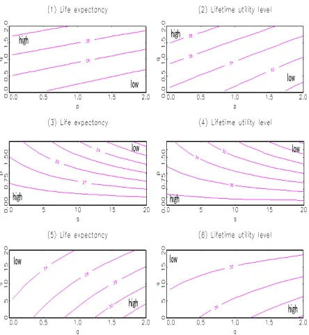
Each panel in Figure 5 shows the results as the contour lines. Figure 5 (1) and 5 (2) show
the results of the life expectancy and the lifetime utility level, respectively, when s is fixed at
10.0 while p and q are changed. In Figure 5 (1) and 5 (2), the values on the left-upper side are
high and the values on the right-lower side are low. Under fixed s, when p is small andq is big,
the life expectancy is longer and the lifetime utility level is higher. Figure 5 (3) and 5 (4) show
the results of the life expectancy and the lifetime utility level, respectively, when q is fixed at 1.0
while p and s are changed. In Figure 5 (3) and 5 (4), the values on the left-lower side are high
and the values on the right-upper side are low. Under fixed q, when p is small and s is short,
Figure 5: Life expectancy and lifetime utility level
the results of the life expectancy and the lifetime utility level, respectively, whenp is fixed at 1.0
while q and s are changed. In Figure 5 (5) and 5 (6), the values on the right-lower side are high
and the values on the left-upper side are low. Under fixedp, whenq is big andsis short, the life
expectancy is longer and the lifetime utility level is higher.
To summarize these results, when pis small, whenq is big, and whensis short, that is, when
of money from his pension, the life expectancy is longer and the lifetime utility level is higher.
The increase in lifetime utility is hardly astonishing because the lifetime budget constraint of
an individual is shifted to the right when an individual receives more benefits from the pension
system and has not to pay for it. These results accord with intuition.
Next, we show the relationship among the life expectancy, the lifetime utility and the pension
system through the combination ofp,q and sand compare them with the results from the cross
section data in Section 2.
21 22 23 24 25 26 27 28 29 30 31 32 33
27.5
30.0
32.5
35.0
37.5
40.0
42.5
Life expectancy
Lifetime utility level
I
II
III
IV
[image:22.595.108.487.252.504.2]A
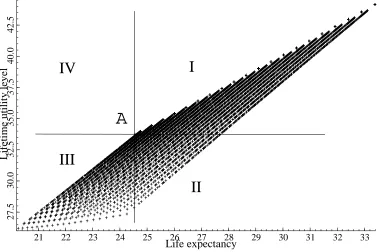
Figure 6: Comparison of the results with and without the pension system
Figure 6 plots the relationship between the life expectancy and the lifetime utility level. By
changing of the paremeters for pension system which are the amount of payment for pension,
the amount of pension gratuity and the period of payment for pension, respectively, we get the
combinations of life expectation and life utility. The horizontal line and the vertical line show
the life expectancy and the lifetime utility level, respectively.6 The +’s in Figure 6 are the
corresponding values of the life expectancy in Figure 5 (1), 5 (3) and 5 (5), and the lifetime utility
level in Figure 5 (2), 5 (4) and 5 (6). And point A (24.556, 33.742) shows the pair of the life
expectancy and the lifetime utility level obtained from the benchmark model. All of these +’s
6The figures of the life expectancy tell nothing about the relative length of life expectancy. As the concept of
except pointAshow the pairs when the pension system exists in some way or another. We draw
a vertical and horizontal line from point A and divide the plain into 4 areas. In area I, the life
expectancy is longer and the lifetime utility level is higher compared to point A. In area II, the
life expectancy is longer but the lifetime utility level is lower compared to point A. In area III,
the life expectancy is shorter and the lifetime utility level is lower compared to point A. There is
no pair in area IV.
The life expectancy is not always proportional to the lifetime utility level. Comparing any ’+’
in area II and pointA, even though the life expectancy is longer, the lifetime utility level is lower.
And the pension system can make life expectancy longer or shorter and can make lifetime utility
level higher or lower. If we get big amounts of pension in the future, the life expectancy can be
extended and the lifetime utility can go up. It is the most preferable, however, in today’s reality,
the pension system cannot avoid the problem of financial resources.
The pension system could also lead to some kind of infirmity as follows: 1) Even though the
life expectancy is extended, the lifetime utility level goes down. By that, an individual is forced to
pay the pension during his young period, the pension system leads to less personal consumption
in his young period. Even though he tries to prolong his life for a long time to get his money back
which he paid mandatorily, his lifetime utility level can go down compared to a case of no pension
system. As rising longevity incited by the pension system, the years they gain in life expectancy
may not be healthy ones, so the increase in life expectancy requires more savings for health-care
spending in his/her old age and less consumption through his/her wholelife. It is also confirmed
from the data in Section 2 that the increase in life expectancy without an increase in income does
not affect too much utility. For example, this is the case of the right shift from point A on the
horizontal line. 2) The life expectancy is decreased, moreover, the lifetime utility level goes down.
This is the worst scenario. An individual can choose a short life to refuse to pay the pension until
such period sand to increase his consumption in his young period.7
The public pension system which is a compulsory savings crowds out the private savings and
can prevent the utility maximization. It is not always true that the pension system improves the
lifetime utility level as shown in area II and III in Figure 6. As we have seen in Section 2 with the
cross section data in the developed countries, the level of happiness and life excpectancy in the
case of no pension system are higher then those in the case with pension system. Not only the
7There was an accident reported in South Korea last 2005, where in a person who was against the compulsory
government has to exert effort to avoid infirmities as stated above, but the government also has
to reconsider about the raison d’etre (the reason for existence) of the compulsory pension system.
Appendix
A.1 Derivation of Eq. (27)
Let us put B =−C−1
1 . Multiplying both sides of Eq. (26) by e−rt and integrating to timet, we get the following
( ˙x−rx+z)e−rt=Be−ρt
xe−rt−z
re
−rt+D
1=−B
e−ρt
ρ +D2
(A1)
whereD1 and D2 are constants of integration. Eq. (A1) can be arranged as follows
xe−rt− z
re
−rt=−Be−
ρt ρ +B
1
ρ +C2
(
x−z
r
)
e−rt=−B(e−
ρt−1 ρ
) +C2
(A2)
whereC2=D2−D1−Bρ1. Multiplying both sides of Eq. (A2) bye−rtand substitutingB=−C1−1
into Eq. (A2), Eq. (A2) can be arranged as Eq. (27).
A.2 Derivation of Eq. (33)
Let us putA= ln(ρx0−(1−e−rT)
z r
1−e−ρT
) .
∫ T
0
e−ρtln(ρx0−(1−e −rT)z
r
1−e−ρT e
(r−ρ)t) dt =
∫ T
0 [
Ae−ρt+ (r−ρ)te−ρt]
dt
=A
∫ T
0
e−ρt dt+ (r−ρ)
∫ T
0
te−ρt dt =A[−e−
ρt ρ
]T
0 −(r−ρ)
[(ρt+ 1)e−ρt
ρ2
]T 0
=−A(e
−ρT −1
ρ
)
−(r−ρ)((ρT+ 1)e−
ρT −1 ρ2
)
(A3)
Substituting A= ln(ρx0−(1−e−
rT)z r
1−e−ρT )
into Eq. (A3), Eq. (A3) can be arranged as Eq. (33).
References
[1] Acemoglu, D., and Johnson, S., 2007. Disease and development: The effect of life expectancy
on economic growth,Journal of Political Economy, Vol.115(6), pp.925-985.
[2] Bloom, D. E., Canning, D., Mansfield, R. K., and Moore, M., 2007. Demographic change,
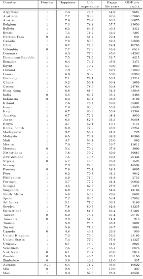
Table 4: Data Set
Country Pension Happiness Life Happy GDP per expectancy life years capita
Argentina 1 7.3 74.8 54.9 9687
Australia 1 7.7 80.9 62.5 37863
Austria 1 7.6 79.4 60.2 36075
Belgium 1 7.3 78.8 57.7 33656
Bolivia 1 6.3 64.7 40.5 3331
Brazil 1 7.5 71.7 53.5 7297
Burkina Faso 0 4.4 51.4 22.4 831
Canada 1 7.8 80.3 62.5 35836
Chile 1 6.7 78.3 52.4 10783
Colombia 0 7.7 72.3 55.8 6514
Denmark 1 8.3 77.9 65.0 34283
Dominican Republic 1 7.5 71.5 53.7 8215
Ecuador 1 6.4 74.7 47.6 5374
Egypt 1 5.7 70.7 40.0 4059
Finland 1 7.9 78.9 62.2 31840
France 1 6.6 80.2 53.0 30952
Germany 1 7.1 79.1 56.3 32214
Ghana 1 5.2 59.1 30.8 1659
Greece 1 6.4 78.9 50.8 24764
Hong Kong 1 6.6 81.9 54.3 32048
India 0 5.5 63.7 35.1 2466
Indonesia 0 6.3 69.7 43.8 3192
Ireland 1 7.6 78.4 59.6 38301
Israel 1 7.0 80.3 55.9 23533
Italy 1 6.7 80.3 53.8 29384
Jamaica 1 6.7 72.2 48.4 8930
Japan 1 6.5 82.3 53.5 30858
Kenya 1 3.7 52.1 19.1 1141
Korea, South 1 6.0 77.9 46.9 22254
Madagascar 1 3.7 58.4 21.8 725
Malaysia 1 6.5 73.7 48.2 10366
Mali 1 4.7 53.1 25.0 862
Mexico 1 7.9 75.6 59.7 11611
Morocco 0 5.4 70.4 37.9 3006
Netherlands 1 7.6 79.2 59.9 36687
New Zealand 1 7.5 79.8 59.5 26436
Nigeria 0 5.7 46.5 26.3 1527
Norway 1 7.9 79.8 62.8 48534
Panama 0 7.8 75.1 58.3 8095
Peru 1 6.2 70.7 44.1 5642
Philippines 1 5.9 71.0 41.8 2753
Portugal 1 5.7 77.7 44.4 20032
Senegal 1 4.5 62.3 27.9 1374
Singapore 1 6.9 79.4 54.6 42103
South Africa 1 5.8 50.8 29.6 6697
Spain 1 7.2 80.5 58.4 27852
Sri Lanka 1 5.1 71.6 36.2 3186
Sweden 1 7.8 80.5 62.9 33235
Switzerland 1 8.0 81.3 65.2 37295
Taiwan 0 6.2 76.4 47.4 26107
Tanzania 0 2.8 51.0 14.4 913
Tunisia 1 5.9 73.5 43.3 5692
Turkey 1 5.6 71.4 39.7 9084
Uganda 0 4.8 49.7 23.9 959
United Kingdom 1 7.2 79.0 56.5 33166
United States 1 7.4 77.9 57.9 41327
Uruguay 1 6.7 75.9 51.0 8927
Venezuela 1 7.5 73.2 55.1 8876
Viet Nam 0 6.1 73.7 45.0 2014
Zambia 0 5.0 40.5 20.1 1156
Zimbabwe 0 3.0 40.9 12.0 337
Average 0.79 6.4 71.2 46.6 16622
Min 0 2.8 40.5 12.0 337
Max 1 8.3 82.3 65.2 48534
[3] Bohn, H., 2009. Intergenerational risk sharing and fiscal policy, Journal of Monetary
Eco-nomics, Vol.56(6), pp.805-816.
[4] Boucekkine, R., de la Croix, D., and Licandro, O., 2002. Vintage human capital, demographic
[5] Boucekkine, R., de la Croix, D., and Licandro, O., 2003. Early mortality decline at the dawn
of modern growth,Scandinavian Journal of Economics, Vol.105(3), pp.401-418.
[6] Chakraborty, S., 2004. Endogenous lifetime and economic growth,Journal of Economic
The-ory, Vol.116(1), pp.119-137.
[7] Cipriani, G. P., 2000. Growth with unintended bequests,Economics Letters, Vol.68(1), pp.51-53.
[8] Cutler, D. M., and Gruber, J., 1996. Does public insurance crowd out private insurance?,
Quarterly Journal of Economics, Vol.111(2), pp.391-430.
[9] de la Croix, D., and Licandro, O., 1999. Life expectancy and endogenous growth,Economics
Letters, Vol.65(2), pp.255-263.
[10] Dushi, I., Friedberg, L., and Webb, T., 2010. The impact of aggregate mortality risk on
defined benefit pension plans,Journal of Pension Economics and Finance, Vol.9(4), pp.481-503.
[11] Feldstein, M. S., and Liebman, J. B., 2002. The distributional aspects of social security and
social security reform, NBER Chapters, pp.263-326. National Bureau of Economic Research,
Inc.
[12] Gorski, M., Krieger, T., and Lange, T., 2007. Pensions, education and life expectancy,
Work-ing Papers Series, No.2007-02, from University of Paderborn, Center for International Eco-nomics.
[13] Krueger, D., and Kubler, F., 2002. Intergenerational risk sharing via social security when
markets are incomplete,American Economic Review, Vol.92(2), pp.407-410.
[14] Lee, R., Mason, A., and Miller, T., 2000. Life cycle savings and demographic transition: the
case of Taiwan, Population and Development Review, Vol.26, Supplement: Population and Economic Change in East Asia, pp.194-219.
[15] Momota, A., Tabata, K., and Futagami, K., 2005. Infectious disease and preventive behavior
[16] Pecchenino, R. A., and Pollard, P. S., 1997. The effects of annuities, bequests, and aging in an
overlapping generations model of endogenous growth,Economic Journal, Vol.107, pp.26-46.
[17] Pecchenino, R. and Pollard, P. S., 2002. Dependent children and aged parents: Funding
education and social security in an aging economy, Journal of Macroeconomics, Vol.24(2), pp.145-169.
[18] Pecchenino, R. A., Utendorf, K. R., 1999. Social security, social welfare and the aging
popu-lation, Journal of Population Economics, Vol.12(4), pp.607-623.
[19] Pestieau, P., and Ponthiere, G., 2012. The public economics of increasing longevity, Review
of Public Economics, Vol.200, pp.41-74.
[20] Ponthiere, G., 2009. Rectangularization and the rise in limit-longevity in a simple overlapping
generations model,The Manchester School, Vol.77(1), pp.17-46.
[21] S´anchez-Marcos, V., and S´anchez-Martin, A. R., 2006. Can social security be welfare
improv-ing when there is demographic uncertainty?, Journal of Economic Dynamics and Control,
Vol.30(9-10), pp.1615-1646.
[22] Shiller, R., 1999. Social security and institutions for intergenerational, intragenerational and
international risk sharing,Carnegie-Rochester Conference Series on Public Policy, Vol.50(1), pp.165-204.
[23] Weil, D. N., 2007. Accounting for the effect of health on economic growth,Quarterly Journal
of Economics, Vol.122(3), pp.1265-1306.
[24] Zhang, J. and Zhang, J., 2004. How does social security affect economic growth? Evidence
from Cross-Country Data,Journal of Population Economics, Vol.17(3), pp.473-500.
[25] Zhang, J., Zhang, J., and Lee, R., 2001. Mortality decline and long-run economic growth,
Journal of Public Economics, Vol.80(3), pp.485-507.
[26] Zhang, J., Zhang, J., and Lee, R., 2003. Rising longevity, educatuion, savings, and growth,