Munich Personal RePEc Archive
Nowcasting Irish GDP
D’Agostino, Antonello and McQuinn, Kieran and O’Brien,
Derry
European Central Bank, Central Bank of Ireland, Central Bank of
Ireland
2011
Online at
https://mpra.ub.uni-muenchen.de/32941/
Nowcasting Irish GDP
∗Antonello D’Agostino † ECB and CBFSAI
Kieran McQuinn‡ CBFSAI
Derry O’Brien§ CBFSAI
July 2011
Abstract
In this paper we present a dynamic factor model that produces nowcasts and backcasts of Irish
quar-terly GDP using timely data from a panel dataset of 35 indicators. We apply a recently developed
methodology, whereby numerous potentially useful indicator series for Irish GDP can be availed of
in a parsimonious manner and the unsynchronized nature of the release calendar for a wide range of
higher frequency indicators can be handled. The nowcasts in this paper are generated by using
dy-namic factor analysis to extract common factors from the panel dataset. Bridge equations are then
used to relate these factors to quarterly GDP estimates. We conduct an out-of-sample forecasting
simulation exercise, where the performance of the factor model is compared with that of a standard
benchmark model.
JEL classification: C33, C53, E52.
Keywords: GDP, Forecasting, Factors.
∗The views expressed in this paper are our own, and do not necessarily reflect the views of the European
Central Bank or the Central Bank of Ireland
†Contact: Contact: European Central Bank, Postfach 16 03 19, 600 66, Frankfurt am Main, Germany;
e-mail: [email protected].
‡
Central Bank and Financial Services Authority of Ireland, PO Box 559 - Dame Street, Dublin 2, Ireland. E-mail:[email protected].
§Central Bank and Financial Services Authority of Ireland, PO Box 559 - Dame Street, Dublin 2, Ireland.
1
Introduction
In this paper early estimates or nowcasts and backcasts of quarterly Irish GDP are presented.
A nowcast (backcast) is a prediction of the present (near past) series with a publication lag.
We draw upon the factor analysis based literature in seeking to distill significant information
from relatively large amounts of variables. The approach follows that of Giannone, Reichlin
and Small (2008) who produce nowcasts of output for the US using a dynamic factor model.
The nowcasting methodology has been applied to many countries including Euro Area
(Angelini et al, 2010), Norway , (Aastveit and Trovik, 2011), Switzerland (Siliverstovs
and Khoodilin, 2010), New Zealand (Matheson, 2011). For a survey of the literature see
Banbura, Giannone and Reichlin (2011).
A nowcast estimate of GDP is obtained in two steps. In the first step, monthly indicators
are used to estimate factors. These factors are then used as regressors in an associated bridge
equation. In the Irish case, we compile a monthly panel dataset of 35 variables. In terms
of the timeliness of Irish GDP releases, for the first two months in any given quarter, the
most recent available release of GDP is for the second last quarter. By the end of the
third month in each quarter, releases of GDP are available for the previous quarter. In
this paper we generate estimates for the current quarter, (nowcast), and for the previous
quarter, (backcast). In the case of the latter, this is only done when no release is available,
i.e. for the first two months of the quarter.
We generate the nowcasts using a pseudo-real time approach. By this, we mean that
when a nowcast is derived from the data in every quarter, the data availability, which existed
at that quarter, is replicated exactly. In essence, we are seeking to replicate the timeliness,
which would have pertained for an analyst at the time the GDP estimate was formulated.
By pseudo we mean that it is the final vintage of this data that is used to produce the
forecasts and not the the “real-time” data available at the time of the forecast, however,
there is evidence that the qualitative results of the model are unaffected by data revisions
(see Liebermann, 2011).
This approach does give rise to what has been referred to as the “jagged edge” issue;
panel from which the factor is derived is unbalanced in nature. In addressing this problem,
we follow the same two-step approach as Giannone, Reichlin and Small (2008), in which
current and recent GDP is estimated conditional on the number of indicators for which
current information is already available.
This modeling approach represents a significant addition to the policy-analysis tool kit
of the Irish Central Bank. The coherent nature of policy making within the Eurosystem
necessitates the provision of timely and accurate estimates of output growth by Member
States. Evaluating the present state of the economy and generating “credible” short-term
forecasts has often been a complex task of combining information from both qualitative and
quantitative based sources usually available at different time delays. Qualitative,
survey-type information concerning present conditions within the economy tends to be available on
a timely and up to date basis, whereas data more typically used in model based forecasts is
often only available at a significant time lag. Additionally, many timely and useful variables
are released at monthly intervals, whereas the variable of interest - GDP is normally on
a quarterly basis. Therefore, from a policy perspective, the flexibility afforded by the
nowcasting model is a particularly attractive feature of this approach.
To place the nowcasting exercise in context, in the next section, we discuss both the type
and timeliness of Irish macroeconomic data releases. In section 3, the nowcasting model
is presented along with the results of an out-of-sample forecast simulation. A final section
offers some concluding comments.
2
Real-time Data Flow and the Indicator Dataset
The Quarterly National Accounts (QNA) releases of the Irish Central Statistics Office (CSO)
provide the most comprehensive available information on recent developments in the Irish
economy. The QNA provide estimates of GDP and its main output and expenditure
com-ponents with the income accounts only available on an annual basis. The current release
delay is no later than 90 days, meaning that GDP growth for a reference quarter is
avail-able towards the end of the subsequent quarter. In view of this significant release delay,
of quarterly GDP of sufficient accuracy and timeliness. Such an early indicator could avail
of the many releases of monthly Irish data.
In order to illustrate more fully the benefits of producing backcasts and nowcasts for
Irish GDP, it is helpful to examine the timeline of releases of Irish macroeconomic data
more carefully. Let’s suppose we are currently half way through a particular quarter and
label the quarterqt. The release of the quarterly national accounts for the previous quarter,
qt−1, will still not appear for another six weeks or so i.e. close to the end of qt. However,
there is considerable monthly information now available for the previous quarter including
monthly releases of retail sales and industrial production for each month of the previous
quarter. This paper proposes to make use of the available monthly information to produce
a timely backcast of GDP i.e. an estimate of GDP for qt−1. At the current juncture
in the middle of qt, there is already partial information available on the current quarter
including the unemployment rate and exchange rate data for the first month of the quarter.
The methodology adopted in this paper also makes use of these monthly data to produce
a timely nowcast of GDP for qt. Such a nowcast yields significant benefits in terms of
providing important timely information on the state of the economy. The official quarterly
national accounts for qt are released at the end of qt+1. The nowcasts and backcasts for
GDP can be computed at any point duringqtbut clearly the nowcasts are more reliable as
we proceed through the quarter when more and more information on monthly indicators
can be incorporated.
The GDP nowcasting model incorporates information from a large set of more timely,
higher frequency indicators that try to capture conjunctural developments in the Irish and
international economies. There are 35 indicator series in the conditioning set. The full list
of indicators along with their respective sources and release delays are presented in Table 1.
These series are part of a larger set of series used by the Central Bank of Ireland in projection
exercises but the series in the conditioning set satisfied a number of additional criteria
including having a sufficiently timely release delay. The series are generally of monthly
frequency and are significantly more timely than the GDP releases, with the longest release
delay for the monthly series at about 40 days. Each of the series must also be sufficiently
end of the sample reflecting the different release delays of the indicators. The structure of
the dataset should be largely the same, at least for the set of monthly series, at each monthly
update of the quarterly GDP nowcast. The model attempts to nowcast year-on-year GDP
growth for a given quarter and the indicator series undergo transformations before entering
the model. Typically, the series are converted to year-on-year growth rates helping to avoid
the excessive volatility of quarter-on-quarter growth rates.
The dataset contains direct measures of economic activity and price dynamics along
with indirect measures such as business and consumer sentiment surveys. The monthly
indicators presented in Table 1 can be broadly grouped in terms of type and release delay
(in brackets) as follows
• Hard data 1 (release delays of less than 10 days) - includes live register of
unemploy-ment benefit claimants, the unemployunemploy-ment rate and car sales
• Hard data 2 (between 20 and 40 days) - includes housing data, retail sales and
indus-trial production
• Price data (within 12 days) - consumer price sub-indices
• Survey data (within 8 days) - Irish consumer sentiment surveys and euro area
con-sumer and business sentiment surveys
• Financial data 1 (at the end of reference month) - euro sterling and euro dollar
ex-changes rates
• Financial data 2 (within 30 days) - monetary aggregates and private sector credit
The importance of developments in trading partners for the Irish economy is captured
by the inclusion of quarterly weighted import demand and competitiveness variables along
with higher frequency indicators such as consumer and business sentiment indicators for the
euro area and euro exchange rate movements vis-`a-vis sterling and the dollar. Sentiment
indicators offer very timely information on conditions in the domestic and international
economies. Exchange rate data are daily but they enter the model as monthly averages.
particularly those sectors with both higher weighting and more volatile outturns. Industrial
output, which accounts for about a quarter of GDP at factor cost, is an important source
of volatility, as illustrated in Table 2. The volatility is particularly pronounced in certain
manufacturing sub-sectors, such as the manufacture of basic chemicals, and this can present
significant challenges in a forecasting context. The overall monthly industrial output index
is included as an indicator.
It is worth noting that the explanatory power of industrial production indices may
be limited by the fact that the monthly industrial production series are not adjusted for
royalties and licence services imports whereas GDP is adjusted as these inputs are not
regarded as value added. In this respect, it is worth observing that the increasing use
of service inputs over time may not be adequately taken into account (data on services
inputs are only available quarterly with the Balance of International Payments, which is
released at the same time as the QNA). Monetary aggregates have been shown to be useful
in short-term forecasting of activity and are also included.
The contribution of the construction sector to GDP growth has undergone significant
changes during this decade and indicators such as housing completions, housing
registra-tions and private sector credit are included to capture activity in the sector. Activity in
the market services sector is accounted for, primarily, by the monthly retail sales and car
sales indices. The inclusion of a range of public finance series was also considered but
un-fortunately the data were not available at a high frequency over a sufficiently long period of
time.1 Altogether, seven subindices of the CPI remained in our final set of indicators after
the various steps of the selection process. Finally, there are two labour market indicators
i.e. the monthly unemployment rate and the numbers on the live register of unemployment
benefit claimants.
1
3
The Model
In this section we outline the dynamic factor model (Giannone, Reichlin and Small (2008))
used to generate the monthly estimates of GDP. The estimation strategy with this approach
is twofold, in the first, a set of factors are extracted from a panel of monthly indicators, in
the second step, the GDP series is projected onto the factors via a bridge equation.
The Giannone, Reichlin and Small (2008) model can be summarized as follows. A vector
of n monthly, stationary (standardized), year-on-year variables xt = (x1,t, x2,t, ..., xn,t)′,
t= 1,2, ..., T is assumed to have the following dynamic factor model characterisation:2
xt=χt+ξt= Λft+ξt (1)
ft= p ∑
i=1
Aift−i+ζt (2)
ζt=Bηt (3)
where xt in eq.(1) is the sum of two orthogonal components, the common component
χt, and the idiosyncratic componentξt. The common component is the product of ann×r
matrix of loadings Λ and ar×1 vector of latent factorsft. The idiosyncratic component is a
multivariate white noise with diagonal covariance matrix Σξ. Factor dynamics are described
in eq.(2), which is a VAR(p). A1, A2, ..., Ap are matrices of parameters andζt∼N(0, BB′),
where B is a (r×q) matrix3 with q≤r;ηt∼N(0, Iq).
In the Appendix, we outline how consistent estimates of the parameters of the model can
be obtained. Using these estimates, the factors can be estimated in the following manner:
ˆ
Ft=proj[Ft|x1, ..., xT; ˆΛ,A,ˆ B,ˆ Σˆξ]
that is, by applying the Kalman filter to the state-space representation obtained by
replacing estimated parameters in the factor representation:
2
T is the last date available in the monthly year-on-year dataset.
3
We assumeB′
xt= ˆΛft+ξt (4)
ft= p ∑
i=1
ˆ
Aift−i+ζt (5)
The Kalman filter can be also used to evaluate the degree of precision of the factor
estimates
Vk =E[(Ft−Fˆt)(Ft−Fˆt)|x1, ..., xT; ˆΛ,A,ˆ B,ˆ Σˆξ].
while, the estimates of the signal and their degree of precision are given, respectively, by
χt=P roj[χt|x1, ..., xT; ˆΛ,A,ˆ B,ˆ Σˆξ] = ˆΛ ˆFt
E(χt−χˆt)2= ˆΛ′V0Λˆ
This framework is adapted to estimate the factors on the basis of an incomplete dataset,
i.e. a dataset which contains some missing values corresponding to data which has not yet
been released. We impose that the variance of the idiosyncratic part of the series with the
missing observation is infinite at time t. This implies that no weight is put on the missing
variable in the computation of the factors at time t.
We define the level of the GDP for a quarter q as the average of latent, monthly
observations of GDP within that quarter,GDPtq = 13(GDPtm+GDPtm−1+GDPtm−2); where
GDPm
t denotes the unobservable latent realization ofGDP at the monthly frequency.
Year-on-year GDP growth is computed as gdpqt = GDPtq −GDPtq−12 within the same quarter
q. Quarterly factors are computed by averaging over the year-on-year monthly factors
ftq = 13(ftm+ftm−1+ftm−2).
The estimates of year-on-year changes of GDP, on quarterly variables, are computed
with the following bridge equation:
d
gdpt q
= ˆβ′fˆtq (6)
where gdpdt q
denotes the yearly estimated growth rate of GDP and ˆβ is ar×1 vector
quarter q. Backcasts, nowcasts and forecasts of the GDP series can be computed every
month as soon as new information becomes available.
The forecast error is defined as the difference between the (ex post) realized and the
estimated value of gdp: εqt =gdpqt −gdpdqt. We assume that εqt ∼N(0, σε2) and that ξt, ζt
andεt are mutually independent at all leads and lags.
3.1 Model Evaluation
To evaluate the forecast performance of the modelling approach, we perform a pseudo
real-time out of sample simulation. In using the pseudo real-real-time approach, we are seeking
to replicate the actual data availability situation, which pertained at the time the
now-cast/forecast is generated. Therefore, the parameters of the model are generated recursively
based on the data availability at a particular quarter.
The out of sample simulation procedure is as follows; the exercise begins by estimating
the model on a sub-sample called the estimation window 1980:Q1 to 1996:Q4. The estimated
parameters are then used to backcast and nowcast GDP. The estimation window is updated
sequentially with one observation and the parameters are re-estimated based on the new
sample available. The estimates of GDP are again generated using the new sample. This
procedure is then iterated until the end of the sample.
We evaluate the performance of the model by generating the Mean Squared Forecast
Error (MSFE), which is defined as
M SF E = 1 (t1−t0+ 1)
t1
∑
t=t0
(gdpqt −gdpdqt)2, (7)
The MSFE refers to Mean Squared Nowcast Error (MSNE) when the evaluation is
computed for the months within the current quarter or refers to Mean Squared Backcast
Error (MSBE) when the evaluation is computed in the months falling in the next quarter.
We also compare the accuracy of the models estimates with that of a benchmark model.4
4
In our case we take, as the benchmark model, the average of the last four most recently
available year-on-year GDP changes. The results in the model simulation are generated with
a specification with one dynamic factor, one static factor and the VAR for the factors of order
4. This specification results in the lowest mean square forecast error in a training sample
from 1990 quarter 1 to 1996 quarter 4 as well as in the sample used for the simulation.5
3.2 Results
We now compare the forecast performance of the model in terms of both nowcasts and
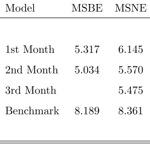
backcasts vis-a-vis that of the benchmark model. Table 3 presents the mean squared errors
(MSE) for the different applications. These are presented for the case where the nowcast
or the backcast is generated for each of the three different months in each quarter.
It can be seen from the Table that in both the case of the backcasts and the nowcasts,
the mean squared backcast error (MSBE) and the mean squared nowcast error (MSNE) of
the benchmark model is considerably greater than the model proposed here. In terms of
the month in the quarter the now/backcast is generated, it is evident, as one would expect,
that as one moves from the first month to the second and onto the third month, there are
notable declines in the MSBE and the MSNE.
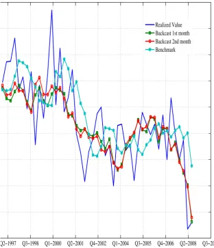
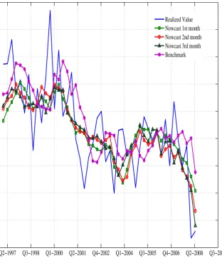
In Figures 2 and 3, we plot the backcast and the nowcast respectively along with the
observed series and the results from the benchmark model. From Figure 2, it may be
observed that the backcast generated for the second month tracks the observed series quite
well, particularly when compared with the estimate of the benchmark. In the case of the
nowcast estimates in Figure 3, the estimate generated for the third month can also be seen
to improve on that estimated in the first and second months of the quarter.
As a final exercise, we examine the effect of individual data releases on the forecast
accuracy of the approach. In Figure 4, we plot the MSFE for the nowcast associated with
the addition of each data release. This is compared with the score for the benchmark. As
with those of the standard benchmark model - the results do not change. They are available, upon request, from the authors.
5
can be seen from Table 1, the first set of available releases contains exchange rates while
the last is for extra euro area demand for Irish exports and competitors’ prices on the
export side. Apart from surveys, a marginal improvement can be observed relative to the
forecasting performance of the previous release. The improvement is particularly notable
for the releases of the live register of unemployment claimants, housing data and monetary
aggregates.
4
Conclusions
The use of the dynamic factor model framework for producing nowcasts and backcasts
represents a significant addition to the forecasting tool kit of the Central Bank of Ireland.
In providing timely estimates of quarterly GDP, the approach has some appealing features.
A large panel dataset of potential indicators for GDP may be parsimoniously employed
through the dynamic factor model methodology and at any time during a quarter the
estimation approach can handle and exploit the unsynchronized flow of generally higher
frequency data.
In evaluating the dynamic factor model, a pseudo-real time approach is followed in that
the data availability situation, which existed for each quarter, is replicated when computing
the model estimates. An out-of-sample simulation is performed where the estimates of the
model are compared with that of a benchmark approach. We find that the mean squared
forecast errors for both the nowcasts and the backcasts are considerably smaller than those
of the benchmark model. Unsurprisingly, the later in the quarter the nowcast or the backcast
is generated, the more accurate the estimate proves to be relative to the observed series.
This suggests that macroeconomic data releases have an important informational content;
it is hence worth updating the forecast many times within the same quarter to incorporate
References
[1] Aastveit, K. and T. G. Trovik (2007). Nowcasting Norweigen GDP: The role of asset
prices in a small open economy, Norweigen Central Bank Working Paper 2007/9.
[2] Angelini E., Camba-Mndez G, Giannone D, Rnstler G and ReichlinL., 2008.
”Short-term forecasts of euro area GDP growth,” Working Paper Series 949, European Central
Bank.
[3] Banbura M., Giannone D. and L. Reichlin, 2010, ”Nowcasting”, chapter in Clements
and Hendry, editors, Oxford Handbook on Economic Forecasting
[4] Giannone, D., L. Reichlin and D. Small (2008). “Nowcasting: The real-time
informa-tional content of macroeconomic data,” inJournal of Monetary Economics, Vol. 55(4), 665-676, May.
[5] Liebermann, J. (2011). Real-time nowcasting of GDP: Factor model versus professional
forecasters, Central Bank of Ireland Research Technical Paper 03/RT/11.
[6] Matheson, Troy D., 2010. ”An analysis of the informational content of New Zealand
data releases: The importance of business opinion surveys,” Economic Modelling,
El-sevier, vol. 27(1), pages 304-314, January.
[7] Siliverstovs B and K. A. Kholodilin, 2010. ”Assessing the Real-Time Informational
Content of Macroeconomic Data Releases for Now-/Forecasting GDP: Evidence for
Switzerland,” Discussion Papers of DIW Berlin 970, DIW Berlin, German Institute for
Economic Research.
[8] Stock, J.H. and M. Watson (2002a). “Forecasting using principal components from a
large number of predictors,” Journal of the American Statistical Association, 97(460), 147-162.
[9] Stock, J.H. and M. Watson (2002b). “Macroeconomic forecasting using diffusion
Appendix A: Parameters Estimation
In this Appendix, we outline how consistent estimates of the parameters of the dynamic
factor model are obtained. Suppose thatzit=yit−µˆiand thatxit= σˆ1i(yit−µˆi), where ˆµ=
1
T ∑T
t=1yt and ˆσi = √
1
T ∑T
t=1(yt−µˆi)2. Consider the following estimator of the common
factors:
( ˜Ft,Λ) = arg minˆ Ft,Λ
T ∑ t=1 n ∑ i=1
(zit−ΛiFt)
2
The correlation matrix of the observables (yt) can be defined as:
S = 1
T
T ∑
t=1
xtx′t
Let’s define D ther×r diagonal matrix with diagonal elements given by the r largest
eigenvalues of S and V the n×r matrix of the corresponding eigenvectors subject to the
normalizationV′V =Ir. Factors are estimated as:
˜
Ft= Λxt
and the factor loadings ˆΛ are estimated by regressing the variables on the estimated
factors: ˆ Λ = T ∑ t=1
xtF˜t′( T ∑
t=1
˜
FtF˜t ′
)−1
and the covariance matrix of the idiosyncratic component is estimated as:
ˆ
Σξ=diags(S−V DV)
The other parameters ˆAand Σ are estimated by running a VAR on the estimated factors:
ˆ A= T ∑ t=2 ˜
FtF˜t′−1(
T ∑
t=2
˜
Ft−1F˜t′−1)− 1
ˆ
Σ = 1
T −1
T ∑
t=2
˜
FtF˜t′−Aˆ(
1
T −1
T ∑
t=2
˜
Ft−1F˜t′−1) ˆA′
Finally, P is defined as the q×q diagonal matrix with the entries given by the largest q
eigenvalues of ˆΣ and by M ther×q matrix of the corresponding eigenvectors, then:
ˆ
Table 1: List of Variables used in the Factor Analysis
Name Frequency Timeliness Source
(approx. days)
Live Register M 10 www.cso.ie/prlabfor.htm
Retail Sales M 40 www.cso.ie/prservices.htm
Car Sales M 10 www.cso.ie/prtransport.htm
Unemployment Rate M 10 www.cso.ie/prlabfor.htm
Industrial Production M 40 www.cso.ie/prind.htm
Real M1 M 30 www.centralbank.ie
Real M3 M 30 www.centralbank.ie
Real Private Sector Credit M 30 www.centralbank.ie
CPI sub-indices (7 series) M 30 www.cso.ie/prprices.htm
House Completions M 20 www.environ.ie/
House Registrations M 20 www.environ.ie/
Consumer sentiment index M 8 www.esri.ie/
Index of consumer expectations M 8 http://www.esri.ie/
Euro sterling exchange rate M 0 www.centralbank.ie
Euro dollar exchange rate M 0 www.centralbank.ie
Euro area consumer and
business surveys (11 series) M 3 http://ec.europa.eu/
Extra euro area demand for
Irish exports Q variable ECB
Intra euro area competitors’
prices on export side Q variable ECB
Table 2: Mean Absolute Deviations of Year-on-Year Growth Rates by Sector
Mean Absolute Deviation Share of GDP
at Factor Cost
Agriculture 28.0 2.3
Industry (excl. Construction) 31.4 25.1
Building and Construction 16.7 8.5
Distribution, Transport
and Communication 8.0 15.6
Public Administration
and Defence 2.4 3.4
Other Services 8.1 46.2
Note: Shares are approximate, due to non-additivity of the chained-linked data, and do not add to
[image:16.595.227.376.521.665.2]100.
Table 3: Mean Squared Errors (MSE) for Backcasts and Nowcasts
Model MSBE MSNE
1st Month 5.317 6.145
2nd Month 5.034 5.570
3rd Month 5.475
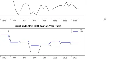
Figure 1: Irish GDP Growth Rates 2000 - 2007
Year-on-Year Rates for each Quarter
%
2000 2001 2002 2003 2004 2005 2006 2007
-2 0 2 4 6 8 10 12 14
Initial and Latest CSO Year-on-Year Rates
%
2 4 6 8 10 12
Inital Latest
Figure 1: Comparison of Backcasting Performance
Q2−1997 Q3−1998 Q1−2000 Q2−2001 Q4−2002 Q1−2004 Q3−2005 Q4−2006 Q2−2008 Q3−2009 Realized Value
Figure 2: Comparison of Now-Casting Performance
Q2−1997 Q3−1998 Q1−2000 Q2−2001 Q4−2002 Q1−2004 Q3−2005 Q4−2006 Q2−2008 Q3−2009 Realized Value
Figure 4
Impact of Data Releases on Forecast Accuracy
0 5 10 15 20 25 30 35