Munich Personal RePEc Archive
Evolution paths on the equilibrium
manifold
Andrea, Loi and Stefano, Matta
University of Cagliari
November 2006
Evolution paths on the equilibrium manifold
Andrea Loi
∗(University of Cagliari)
Stefano Matta
†(University of Cagliari)
November 2006
Abstract: In a pure exchange smooth economy with fixed total resources, we de-fine the length between two regular equilibria belonging to the equilibrium manifold as the number of intersection points of the evolution path connecting them with the set of critical equilibria. We show that there exists a minimal path according to this definition of length.
Keywords: Equilibrium manifold, regular economies, critical equilibria, catastro-phes, Jordan-Brouwer separation theorem.
JEL Classification: D50, D51, D52, D80.
∗Dipartimento di Matematica e Informatica, Universit`a di Cagliari, Italy, E-mail: [email protected] †Correspondence to S. Matta, Dipartimento di Economia, Universit`a di Cagliari, viale S.
1
Introduction
The equilibrium manifold (E henceforth) is defined as the set of pairs of price vectors and endowments such that the aggregate excess demand function is equal to zero. The global and local topological structure of the set E has been deeply investigated by Balasko (see [1] and his monograph [4]). One of the global topo-logical properties of this set, which we are concerned with in our analysis, is the arc-connectedness property. This property has a straightforward economic mean-ing: let ω and ω′ be two m-tuples of initial endowments and let p and p′ be two
equilibrium price vectors associated withω andω′, respectively. Then there exists
a continuous modification (ω1(t), . . . , ωm(t)), t ∈ [0,1], from the m-tuple of ini-tial endowments ω to ω′ such that for every t there is an equilibrium price vector p(t) associated with (ω1(t), . . . , ωm(t)) andp(t) is a continuous function, p(0) =p
and p(1) = p′. Observe that there exist infinite trajectories connecting two given
equilibria. Furthermore, the spaceE also enjoys the property of being simply con-nected, i.e., it is always possible to deform continuously a continuous trajectory linking two equilibria, (p, ω) and (p′, ω′), to another one linking the same equilibria
(see Section 4 in [1]) and still lying onE.
In his monograph ([4] p. 69) Balasko observed that, under the assumption that the initial and final equilibria (p, ω) and (p′, ω′) are exogenously determined,
a continuous evolution path from the initial to the final state (p′, ω′) should be
considered preferable, from an economic point of view, to any discontinuous one, being discontinuity synonymous of catastrophes. The motivation of our analysis is based on the natural question raised by Balasko ([4] p.70) of choosing one path to follow in the equilibrium manifold E to move from (p, ω) to (p′, ω′). In this
paper we tackle this question. As Balasko observed, one of the most natural ideas would be to minimize length (i.e. to choose the shortest path). But then a new problem arises: according to which metric can one define a distance on the equilibrium manifold? In order to avoid the complication arising from the definition of a metric economically meaningful (see [10, 9]), it can be observed that the same argument which has led to prefer a continuous evolution path also suggests us to choose “regular” paths, namely paths which “avoid” as much as possible the set of critical equilibria. In fact we recall that only the set of regular equilibria is characterized by the desirable economic properties of local uniqueness of equilibria, of the continuity of the equilibrium price correspondence and of the possibility of comparative statics analysis (see [6]). If the path should cross the set of critical equilibria, all these properties could be lost giving rise to catastrophes
minimizes distance) is identified with the one less catastrophic.
This consideration also suggests us to be concerned with the codimension one stratum of critical equilibria (S1 henceforth). The reason is that S1 is the only stratum of critical equilibria which can disconnect E(r). This means that if the evolution path should link two regular equilibria belonging to two disconnected components of E(r)\S1, it would cross S1. On the contrary, it is evident that there always exists a path connecting two regular equilibria belonging to the same connected component of E(r) \ S1 which does not intersect the set of critical equilibria. A natural aspiration, when dealing with equilibria belonging to different connected components, would be to find a path containing at most one critical equilibrium. Unfortunately this event crucially depends on the structure of the set of critical equilibria Ec(r) (see Theorem 2.1). In the more general case, being the setS1 composed by a union of closed smooth manifolds, the equilibrium manifold is divided into several connected components. According to our definition of length, we can say that two equilibria belonging to the same connected component have distance zero, two points separated by only one stratum of critical equilibria have distance one, and so on...
In this paper we show that there exists a path connecting the equilibria which realizes the distance (see Theorem 3.7). As we will see, the possibility of defining the above distance deeply relies on the Jordan-Brouwer separation theorem (see Theorem 3.2), a standard result in differential topology.
Some features that characterize our analysis deserve a few comments. First, total resources are assumed to be fixed. This means that Pmi=1ωi = r, where
r∈Rl is a fixed vector. Then the equilibrium manifold is defined as
E(r) ={(p, ω)∈S×Ω(r)|
m
X
i=1
fi(p, p·ωi) =r},
where S is the set of normalized prices, Ω(r) is the space of economies and
Pm
i=1fi(p, p·ωi) is the aggregate demand function (see Section 2 below). Sec-ond, in our construction we heavily rely on the very nice topological properties enjoyed by the set of critical equilibria Ec(r), this set being a finite and disjoint union of closed smooth submanifoldsSi ofE(r) (see [3, 4] or Theorem 2.1 below). This paper is organized as follows. Section 2 recalls the economic setting. Section 3 contains our definitions and main results.
2
The economic setting
We consider a pure exchange economy with l goods and m consumers. Let S =
Ω = (Rl)m denote the space of endowmentsω= (ω1, . . . , ωm),ωi ∈Rl. We assume
that the standard assumptions of smooth consumer’s theory are satisfied (see [4] Chapter 2). The problem of maximizing the smooth utility function ui :Rl → R subject to the budget constraint p·ωi =wi gives the unique solutionfi(p, wi), i.e. consumer’s i demand. Let E be the closed set consisting of pairs (p, ω) ∈ S×Ω satisfying the following equations:
m
X
i=1
fi(p, p·ωi) = m
X
i=1
ωi.
The setE is a smooth submanifold of S×Ω globally diffeomorphic to (Rl)m (see
[4]). Letπ :E →Ω be the natural projection, i.e. the smooth map defined by the restriction to E of (p, ω)7→ω. Let Ec be the set of critical equilibria, namely the pairs (p, ω)∈E such that the derivative ofπat (p, ω) is not onto. We now analyze the fixed total resources setting. Let r ∈ Rl denote the vector representing the
total resources of the economy and Ω(r) denote the space of economies associated with the fixed total resources, i.e., Ω(r) ={ω ∈(Rl)m|Pm
i=1ωi =r}. Define
E(r) ={(p, ω)∈S×Ω(r)|
m
X
i=1
fi(p, p·ωi) =r},
denote by π : E(r) → Ω(r) the restriction of the natural projection to E(r) and by Ec(r) the set of critical points of π. It can be shown (see [4]) that (p, ω) is a critical equilibrium with respect to π : E(r) → Ω(r) if and only if it is a critical equilibrium with respect to π : E → Ω. The set of critical equilibria when total resources are fixed is denotedEc(r). The structure of E(r) andEc(r) is described in the following theorem where we summarize some results due to Balasko (see [3] and [4]).
Theorem 2.1 (Balasko) E(r) is a smooth manifold globally diffeomorphic to
Rl(m−1) and E
c(r) is a disjoint union of closed smooth submanifolds Si, i = 1, . . . ,inf(l −1, m−1) of E(r). The manifold Si has dimension l(m− 1)−i2
and Si =∅ for i >inf(l−1, m−1).
We will refer to the decomposition Ec(r) = ∪iSi, given by the previous theo-rem, as Balasko’s stratification of the set of critical equilibria Ec(r). The closed manifoldsSi will be called thestrataof this stratification. Observe that for a fixed
i the manifold Si could not be connected. Denote by Sj
i
3
Main results
In the sequel we identify, without further comments, the equilibrium manifoldE(r) with the Euclidean space Rn, n = l(m−1), via Balasko’s theorem 2.1. Observe also that the structure ofEc(r), as defined by the same Theorem 2.1, entitles us to define a smooth path γ : [0,1]→E(r), connecting two regular equilibria in E(r),
transversal to Ec(r) if it intersects each stratum Si transversally.
We refer the reader to Section 5 of Chapter 1 and to Chapter 2 in [7] for the standard material about transversality theory. Actually, the only results about this theory used in this paper are the following three facts and the Lemma 3.1 below.
(i) Two submanifolds X and Z of Rn are said to be transversal, if for every
point x∈X∩Z the following holds (see Section 5, Chapter 1, in [7]):
TxX+TxZ =TxRn =Rn;
(ii) IfX andZ are two transversal submanifolds of Rn, thenX∩Z is a
submani-fold ofRn. Moreover the codimension ofX∩Z inRnequals the codimension
ofX inRn plus the codimension ofZ inRn (see theorem on page 30 in [7]); (iii) (Transversality Theorem) Let X and Z be two closed submanifolds of Rn.
Then there exists an arbitrary small vector s∈Rn (i.e. the Euclidean norm of s can be taken arbitrary small) such that the manifold
X+s ={y∈Rn| y=x+s, x∈X}
intersectsZ transversally. In particular (by (ii)) (X+s)∩Z is a submanifold of Rn (see Section 3, Chapter 2, and the discussion on page 69 in [7]).
In this paper we are only concerned with the intersection between a stratum Si (i.e. a submanifold of E(r) of codimension i2) and the image Imγ =γ([0,1]) of a path γ : [0,1]→E(r) (i.e. a submanifold of E(r) of codimension n−1). With a slight abuse of language, we will say that γ intersects (transversally) the stratum
Siif Imγ intersects (transversally)Si. By (i) above,γ is transversal toSi, for fixed
i, if for every intersection point x0 = γ(t0), t0 ∈ [0,1], between Imγ and Si the tangent vector γ′(t0) ofγ(t) together with Tx0Si generate a n-dimensional space,
being n =l(m−1) the dimension of E(r). Hence a path γ is transversal to Si in the following two cases:
2. the codimension of Si is one, (i.e. i = 1), γ intersects S1 in a finite number of points and for each of these points, say x0 =γ(t0), t0 ∈[0,1], the tangent vectorγ′
(t0) does not belong toTx0S1. In this second case Imγ∩ S1 consists
of a finite number of points since, by (ii) above, Imγ∩S1 is a zero dimensional compact manifold.
The following lemma applies the previous results of transversality theory to a path joining two regular equilibria on the equilibrium manifold.
Lemma 3.1 Given two regular equilibria x, y ∈E(r), there exists a smooth path
γ joining them and intersecting Ec(r) transversally. Such a path does not inter-sect Si for i > 1 and intersects a finite number, say S11, . . . ,S1k, of the connected
components of S1, each one in a finite number of points.
Proof: Take any smooth path σ : [0,1] → E(r) joining x with y (σ exists since
E(r) is connected) and let p = inf(l −1, m −1) (cf. Theorem 2.1). We will prove the theorem by an induction argument on p. Let p = 1. By applying the Transversality Theorem to X = Imσ and Z =S1 we can find a vector s in E(r) such that Imσ+s intersects S1 transversally. By taking s sufficiently small, we can assume that x+s and y+s are regular and there exist smooth paths σ1 and
σ2 joining x with x+s and y+s with y, respectively, which do not intersect S1. The path γ is obtained by suitably smoothing the path σ1∪(σ+s)∪σ2 around the points x+s and y+s, where σ +s : [0,1] → E(r) is the path defined as (σ+s)(t) =σ(t) +s. Assume by induction we have found a path ˜γ : [0,1]→E(r) joining xand y and intersecting each S1, . . .Sp−1 transversally (in a finite number of points). Letx1 = ˜γ(t1) (resp. x2 = ˜γ(t2)) be the first point (resp. the last point) where ˜γ intersects the stratum Sp. Since the strata of Balasko’s stratification are disjoint and closed we can find a sufficiently small δ such thatxδ = ˜γ(t1 −δ) and
yδ = ˜γ(t2 +δ) are regular and ˜γ restricted to [t1 −δ, t2 +δ] does not intersect
∪p−1
j=1Sj. Call this restriction β. By applying again the Transversality Theorem, to Imβ and Sp we can find a vector s ∈ Rn such that Imβ +s is transversal to
Sp. By taking this vector sufficiently small, we can assume that Imβ+sdoes not intersect ∪p−1
j=1Sj and we can find smooth paths β1 and β2 joining xδ with xδ +s and yδ+s with yδ, respectively, which do not intersect Ec(r) =∪
p
j=1Sj. Consider the continuous path ˜γ1∪β1∪(β+s)∪β2∪γ˜2, where β+s : [0,1]→E(r) is the path defined as (β+s)(t) = β(t) + s and ˜γ1 and ˜γ2 denote the restriction of ˜γ to the interval [0, t1−δ] and [t2+δ,1]. Finally, by suitably smoothing this path around the points xδ, xδ+s, yδ+s, yδ, we get the desired path γ. The last part of
the lemma follows by 2.) above.
Theorem 3.2 (Jordan-Brouwer) Let S be a closed, connected, codimension one submanifold of Rn. Then Rn\S consists of two disjoint connected open sets,
R1 and R2, which have S as common boundary.
The proof of the previous theorem can be found in Section 5 of Chapter 2 in [7] under the stronger assumption that the manifold S is compact. The proof of Theorem 3.2, namely when S ⊂ Rn is only assumed to be closed (not necessarily
bounded), is available in Lima’s paper [8] (the authors do not know any text-book where this standard differential topology theorem is proved in the closed case). Actually Lima first proved the Jordan–Brouwer separation theorem for compact manifolds S ⊂Rn but in the concluding remark on page 41 of [8], he indicates a way to prove this theorem under the weaker assumption that S is closed in Rn.
Let S ⊂ Rn be as in the previous theorem and let γ : I → Rn be a smooth
curve connecting x and y inRn\S, namely γ(0) =x and γ(1) = y. Assume that
γ intersects S transversally. Then Imγ∩S is a (possibly empty) zero dimensional manifold and hence it consists of isolated points which are forced to be finite for the compactness of Imγ ∩ S. Observe, by Theorem 3.2, that the parity of Imγ∩S depends on the location ofxand y. More precisely, we have the following straightforward corollary of Theorem 3.2.
Corollary 3.3 Let S ⊂Rn, R1 and R2 be as in Theorem 3.2 and let γ : [0,1]→ Rn be a smooth path joining x and y in Rn\S and intersecting S transversally.
Then the parity of Imγ∩S is even if and only ifxand yboth belong to R1 or they
both belong to R2. In particular, if such a path intersectsS in a single point, then
x and y belong to different connected components of Rn\S.
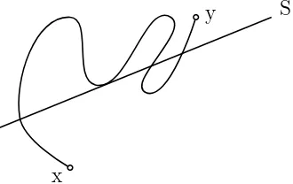
S
x
[image:8.612.244.409.477.581.2]y
Figure 1: Violation of the transversality property
A tool used in the following lemma, which represents a technical result needed to prove our main theorem, is the existence of a smooth unitary normal vector fieldn :S→ Rn on a closed and connected codimension one submanifold S ⊂Rn, namely a smoothRn-valued function on S such that n(s) is perpendicular to T
sS and|n(s)|= 1,∀s ∈S. It can be proved that the existence ofnis equivalent to the
orientability of S (see Section 2, Chapter 3, in [7]). Observe that, once a smooth unitary vector field n on S is given, then −n : S → Rn defines another unitary smooth vector field on S and, by Jordan-Brouwer separation theorem, the vectors
n(s)(resp. −n(s)) point towards either R1 (resp. R2) or R2 (resp. R1), where R1 and R2 are the connected components of Rn\S as in Theorem 3.2. When S is compact, the proof of its orientability can be found in [7], Ex. 13 and 18, on page 104 and 106, respectively. We refer the reader to [11] for an elegant and concise proof of the orientability of S in the closed case.
Lemma 3.4 Let S ⊂Rn be a closed and connected codimension one submanifold
of Rn, let C be a closed set such that S ∩C = ∅ and let σ be a smooth curve
joining two points in the complement of S ∪C which does not intersect C and which intersects S transversally. Then there exists a smooth curve γ joining the given points which does not intersect C and which intersects S transversally in at most one point.
Proof: Let x1 = σ(t1), . . . , xk = σ(tk), with t1 < . . . < tk, be the intersection points of σ with S. Assume k ≥ 2, otherwise there is nothing to prove. We will show that there exists a smooth curve, ˜σ, joining x and y, disjoint from C, and intersecting S transversally inx3, . . . , xk (actually ˜σ will be constructed in such a way to coincide with σ in [0, t1 −δ] and [t2 +δ,1], for a suitable chosen δ). By iterating this procedure, this yields the existence of the desired path γ and, hence, the proof of the lemma. In order to construct ˜σ, let β : [0,1]→S be any smooth curve onS joining x1 =β(0) and x2 =β(1) (β exists since S is connected). Take a smooth unitary normal vector field n:S →Rn onS pointing towardR1, where
R1 is the connected component of Rn\S where x belongs to. Take a positive real number λ, 0 < λ < r, where r denotes the distance between Imβ and C. Then the curve λn(β(t)) is a smooth curve on R1 not intersecting C such that
λn(β(0)) = λn(x1) and λn(β(1)) = λn(x2). For δ and ǫ sufficiently small positive real numbers, the distance betweenxδ =σ(t1−δ) andǫλn(x1) (resp. yδ =σ(t2+δ) and ǫλn(x2)) is arbitrary small (indeed, these distances go to zero as δ, ǫ → 0). Hence we can connect xδ with ǫλn(x1) and ǫλn(x2) with yδ with line segments β1 and β2, respectively, in such way that Imβ1 and Imβ2 belong to R1 and do not intersect C. Then the continuous path α = σ1∪β1 ∪(ǫλn(β))∪β2∪σ2, where
smoothing the pathαaround the pointsxδ, ǫλn(x1), ǫλn(x2), yδ, we get the desired
path ˜σ.
In our economic setting, let γ : [0,1] → E(r) be a smooth path joining two regular equilibria x and y in E(r)\Ec(r). The length of γ, denoted by ℓ(γ), is defined as the number of intersection points of Imγ withEc(r). Observe that ifγ
intersects Ec(r) transversally, then ℓ(γ) is a non negative integer which is zero iff Imγ∩Ec(r) = ∅.
We define the distance,d(x, y), between two regular equilibria x, y ∈E(r)\Ec(r) as the infimum ofℓ(γ), whenγ is varying amongst all the smooth curves joining x
andy. We define a pathγ minimal ifℓ(γ) =d(x, y). By the above considerations,
d(x, y) is always a nonnegative integer.
Remark 3.5 It is worth pointing out that d(x, y) does not define a metric space structure onE(r)\Ec(r). The distance between two regular equilibriax, y belong-ing to the same connected component of E(r)\Ec(r) is zero even if x 6= y. On the other hand, one can define an equivalence relation ∼ on X = E(r)\Ec(r), by defining x∼y iff x and y belong to the same connected component of X. We denote with X/∼ the quotient space and with [x] the equivalence class of x. The
function
e
d:X/∼×X/∼ →N⊂R,
defined byde([x],[y]) =d(x0, y0), wherex0 and y0 are any two regular equilibria in the class of [x] and [y], respectively, is well defined, namely it does not depend on the choice of x0 ∈[x] and y0 ∈[y]. Moreover it is immediate to verify that (X,de) is a metric space.
The following proposition describes a sufficient condition for a pathγinE(r) to be minimal. Letγ : [0,1]→E(r) be a smooth curve joining two regular equilibria
x, y ∈E(r)\Ec(r) and assume thatγ is transversal toEc(r), namely Imγ does not intersect the codimension > 1 strata and intersects transversally a finite number of the connected components ofS1, sayS1j, j = 1, . . . k, in a finite number of points (see Lemma 3.1).
Proposition 3.6 Take γ as above and assume it intersects transversally each
S1j, j = 1, . . . k, in at most one point. Then γ is a minimal path.
Proof: If ℓ(γ) = 0 there is nothing to prove. Let l=ℓ(γ)>0 and letSj1
1 , . . . ,S jl
1 be the connected submanifolds ofS1 intersected transversally exactly in one point by γ. Assume by contradiction that there exists another path in E(r), say σ, joiningxandyand such thatℓ(σ)< ℓ(γ). Then it must exist an indexj0,1≤j0 ≤
l, such that Imσ does not intersect Sj0
1 . This implies that x and y belong to the same connected components of E(r)\Sj0
x and y and intersecting Sj0
1 transversally only in one point. Hence, Corollary 3.3, applied to the closed and connected codimension one submanifold S =Sj0
1 ⊂
E(r) = Rn, implies thatxandybelong to the two different connected components of E(r)\Sj0
1 , which is the desired contradiction. Our main result is the following theorem which asserts the existence of a min-imal path joining two given regular equilibria.
Theorem 3.7 Given two regular equilibria x and y, there exists a smooth curve
γ : [0,1]→E(r), γ(0) =x and γ(1) =y, such that ℓ(γ) = d(x, y).
Proof: Take any curve ˜σ joining x and y and intersecting Ec(r) transversally, whose existence is guaranteed by Lemma 3.1, and let S1
1, . . . , S1k be the number of connected components of S1 intersected by Im ˜σ (observe that Im ˜σ∩ Si is empty for i >1). From Proposition 3.6 the theorem will be proved if there exists a path
γ which intersects each of the manifolds S1
1, . . . , S1k transversally in at most one point and does not intersect Ec(r) in any other point. We construct such a path by an induction argument on the numberk of the previous submanifolds. The case
k = 1 follows by applying Lemma 3.4 toS =S1
1 and to the closed setC =Ec(r)\
S1
1. Assume by induction we have found a path σ which intersects S11, . . . , S1k−1 transversally in at most one point. If Imσ does not intersect S1
1 ∪. . .∪S1k−1, the proof of the theorem follows by applying again Lemma 3.4 to the path ˜σ, S =Sk 1 and C =Ec(r)\S1k. Otherwise, letS
j
1, j ≤k−1, be the last manifold intersected transversally exactly in one point, say ¯x = σ(¯t), by Imσ. For small δ ∈ R, the
point ¯xδ = σ(¯t+δ) is regular. By applying Lemma 3.4 to the path σ restricted to [¯t+δ,1],C =Ec(r)\Sk
1, S =S1k, we get a path ¯γ which does not intersect C, which intersects Sk
1 transversally in at most one point and which connectsxδ with
y. Consider the continuous path ¯σ∪¯γ, where ¯σ is the restriction of σ to [0,¯t+δ]. This path intersects Ec(r) only in the submanifolds S1
1, . . . , S1k and each of them transversally in at most one point. By suitably smoothing this path around the
point xδ, we get the desired pathγ.
References
[1] Y. Balasko, The graph of the Walras correspondence, Econometrica, 43 (1975),
907-912.
[2] Y. Balasko, Economic equilibrium and catastrophe theory: an introduction, Econo-metrica, 46(1978), 557-569.
[4] Y. Balasko, Foundations of the Theory of General Equilibrium, Academic Press, Boston (1988).
[5] Y. Balasko, The set of regular equilibria, J. of Economic Theory 58(1992), 1-8.
[6] E. Dierker, Regular Economies, Chap.17 in Handbook of Mathematical Economics, vol.II, edited by K. Arrow and M. Intriligator. Amsterdam: North-Holland(1982).
[7] V. Guillemin and A. Pollack, Differential Topology, Prentice Hall, Englewood Cliffs (1974).
[8] E.L. Lima,The Jordan-Brouwer separation theorem for smooth hypersurfaces, Am. Math. Monthly 95(1988), 39-42.
[9] A. Loi, S. Matta, A Riemannian metric on the equilibrium manifold: the smooth case, Economics Bulletin 4 No. 30 (2006), 1-9.
[10] S. Matta,A Riemannian metric on the equilibrium manifold, Economics Bulletin4
No. 7 (2005), 1-7.
[11] H. Samelson,Orientability of Hypersurfaces inRn, Proc. Am. Math. Soc.22(1969),