A Monetary Approach to Exchange Rate Dynamics in Low Income Countries: Evidence from Kenya

Munich Personal RePEc Archive

A Monetary Approach to Exchange Rate

Dynamics in Low-Income Countries:

Evidence from Kenya

Nandwa, Boaz and Mohan, Ramesh

Bryant University

2 November 2007

Online at

https://mpra.ub.uni-muenchen.de/5581/

A Monetary Approach to Exchange Rate

Dynamics in Low-Income Countries:

Evidence from Kenya

Boaz Nandwa*

Yale University

Ramesh Mohan

Bryant University

Abstract

The flexible price monetary model assumes that both the purchasing power parity (PPP) and uncovered interest parity (UIP) hold continuously. In addition, the model posits that money market equilibrium exists, which helps to determine the exchange rate. This paper explores exchange rate determination in low-income economies by applying a monetary model to Kenya to examine the exchange rate dynamics in a post-float exchange rate regime. We apply a multivariate cointegration and error correction model (ECM) to investigate whether the long-run exchange rate equilibrium and the rate of adjustment to the long-run equilibrium hold, respectively. Finally, we evaluate the relative performance of ECM versus a random walk framework in the out-of-sample forecasting. We find that the random walk performs better than the restricted model.

Key words: Exchange rate, volatility, regime changes and Kenyan Shilling

JEL classification: C32, C53, E58, F31

______________________________

* Correspondence: Boaz Nandwa, Economic Growth Center, Yale University, 27 Hillhouse Avenue, New Haven, CT 06511. E-mail: [email protected]

A Monetary Approach to Exchange Rate

Dynamics in Low-Income Countries:

Evidence from Kenya

Abstract

The flexible price monetary model assumes that both the purchasing power parity (PPP) and uncovered interest parity (UIP) hold continuously. In addition, the model posits that money market equilibrium exists, which helps to determine the exchange rate. This paper explores exchange rate determination in low-income economies by applying a monetary model to Kenya to examine the exchange rate dynamics in a post-float exchange rate regime. We apply a multivariate cointegration and error correction model (ECM) to investigate whether the long-run exchange rate equilibrium and the rate of adjustment to the long-run equilibrium hold, respectively. Finally, we evaluate the relative performance of ECM versus a random walk framework in the out-of-sample forecasting. We find that the random walk performs better than the restricted model.

Key words: Exchange rate, volatility, regime changes and Kenyan Shilling

1.0 INTRODUCTION

In the analysis of financial markets, the foreign exchange market is arguably the

largest market in the world. This explains the vast interest and literature in analyzing the

determinants, trends and forecasting of the exchange rate series. Generally, exchange

rates play an important role in the global economy in determining relative prices of goods

and services and relative prices of assets in different countries. Further, under the flexible

exchange rate regime, the exchange rate can be influenced, and consequently it has

influence on trade account balances and capital account balances. In many theoretical

models of open macroeconomics the exchange rate is regarded as one of the endogenous

variables of a large macroeconomic system and as an asset price in international finance.

The former implies that the exchange rate is a slow-moving variable similar to

consumption, investment and prices of goods and services, while the latter implies that it

is a fast-moving variable just like stock prices. Hence, for small open economies the

mismatch of the speeds of adjustment can be exploited to produce a result such as the

overshooting model by Dornbusch (1976).

Over the years, attempts to produce a valid long-run equilibrium relationship,

also referred to as purchasing power parity (PPP), as implied by the monetary model,

have generally met with mixed success - particularly when the implicit restrictions of the

model are applied. For instance, Meese (1986) and McNown and Wallace (1989) fail to

find a valid long-run relationship for the conventional monetary model. However,

Macdonald and Taylor (1993) report that the flexible price monetary model appears to

hold as a long-run equilibrium condition in explaining the Deutsche-mark and the US

analyzing PPP under the Balassa–Samuelson effects for small open economies can be

explained by several factors. First, growth in these economies may be propelled by factor

accumulations rather than productivity growth.2 Second, the productivity growth may

have been more uniform across tradables and non-tradables, while relative prices between

these two may have stayed relatively constant in some of the developing economies. This

implies that the PPP for tradables, an assumption central to the Balassa–Samuelson

model, may have been violated. Even prices of tradables may rise in comparison with the

industrialized countries because the compositions of tradables may quickly shift to more

value-added and high-quality products, while adjustments for compositional or quality

changes are not reflected in the data. Third, ambiguity in making clear-cut distinction

between tradables and non-tradables exists. For instance, commonly assigning services

and construction to non-tradables may not be right for service-oriented economies in

some countries. Finally, foreign exchange restrictions may be loosened over the sample

period, so that the artificial overvaluation may be corrected over time. This means that

PPP may not hold if there is no controlling for any structural break in the time series.

Although the monetary model was the first approach applied in explaining the

related phenomenon of exchange rate variations, its application is mostly confined to

analyzing industrialized countries, whereas applications in emerging and low-income

economies are limited. This paper is aimed at testing robustness of the monetary model

for a small open economy by applying it to Kenya over 1990-2006, the period after it

The rest of the paper is structured as follows: section II gives an overview of the

flexible price model, data and estimation methodology. Section III discusses the

empirical results, followed by the conclusion in section IV.

2.0 METHODOLOGY

The monetary approach to exchange rate is based on two foundations: the quantity

theory of demand for money (QTM) and the PPP relationships. The QTM posits that the

demand for real balances is a stable function of only a few variables in the domestic

economy. Thus any change in the nominal money stock will have a direct effect on the

price levels, because velocity of circulation and output are assumed to be constant (a

doubling of the nominal money stock will result in doubling of the price level at any

given real income). On the other hand, the PPP relationship is often tested as a theory to

determine the exchange rate dynamics. In its absolute version, PPP implies that the

equilibrium exchange rate equals the ratio of domestic to foreign prices. On the other

hand, the relative version of PPP relates changes in the exchange rate to changes in the

price ratios. Slow convergence to the PPP relationship is often called the “PPP puzzle”.

The standard money demand function can be specified as

t t t t

m = p + α y − β i (1)

where m is the nominal demand for money, p is the domestic price level, y is the real

income level and i is the nominal rate of interest. All variables, except the interest rate,

are in logarithms. Foreign money demands are given by

* * *

*

t t t t

where * denotes foreign variable. It is assumed that absolute purchasing power parity

(PPP) holds, so that

p

=

p

+

e

where e is the log of the nominal exchange rate. PPP is used only as a long-run

equilibrium condition in this model; in the short run the error correction model allows

deviations from PPP. The evidence on PPP as a long-run equilibrium condition is

generally positive (Culver and Papell, 1999).

Substituting and rearranging equations (1) - (3) yields

* * *

0 1( ) 2( ) 3( )

t t t t t t t

e =

α

α

α

α

The monetary approach assumes that domestic and foreign bonds are perfect substitutes

so that Uncovered Interest Parity (UIP) holds.

]

)

|

(

[

t

i

E

e

I

e

i

=

+

−

where E e( _t+1/I_t) is the rational expectation of the exchange rate one period ahead,

conditional on the currently available information set, I_t. By denoting the set of forcing

variables as Zt [α0 α1(mt mt) α2(yt yt)]

∗ ∗

= + − − − , substituting (5) into (4) and solving for

the exchange rate yields

(

)

(

)

t j t

t t t

E Z I

e

α

α

α

+

+

= +

+ + (6)

Solving this equation by forward iteration gives

(

)

1 3

3 3 3

0 3

(1 ) [ /(1 )] ( | )

1

n n

j

t t j t t n t

j

e α α α E Z I α E e I

α

−

+ +

=

= + + +

Letting j→∞ (or assuming that the solution is free from arbitrary speculative bubbles)

gives the forward-looking solution for the monetary exchange rate (FLME):3

1

3 3 3

0

(1 ) [ /(1 )]j ( | )

t t j t

j

e

α

α

α

∞ −

+ =

= + + (8)

As outlined in Campbell and Shiller (1987) and Macdonald and Taylor (1993), the

exchange rate should be cointegrated with the forcing variablesZ_t. This is illustrated by

subtracting Zt from both sides of equation (7) to obtain

(

)

(

)

(

)

(

)

1 ₃ 3 2

2 3 1 2 3 3 3 3 + + + + + + − =

− _{t t t+ t t+ t}

t Z X E X I E X I

e α α α α α α (9)

Rearranging into first differences (for all j→ ∞) yields

3 3

1

[ /(1 )]j ( | )

t t t j t

j

e Z

α

α

∞

+ =

− = + ∆ (10)

Under rational expectations the forecasting errors are stationary; thus if the forcing

variables in Z_t are I(1), then the right hand side of equation (10) must also be stationary.

Consequently if e_t is also I(1), then the exchange rate must be cointegrated with the

variables m m y_t, *_t, _tandy_t*.

Thus FLME is to test for cointegration between the exchange rate and the forcing

variables.4 Hence the monetary approach to the exchange rate model to be estimated is

given by:

* *

0 1 2 3 4

t t t t t

e

=

β

+

β

m

+

β

m

+

β

yt

+

β

y

+

u

where u_tis a random error term and,

β

β

β

β

. 0 ,

0 _{2 3}

4

1

β

β

β

According to the portfolio approach, the rise in wealth ought to facilitate an

increase in the demand for money and a rise in the interest rate. In the process, higher

interest rates should encourage more capital inflow, and increased demand for the

domestic currency, which results in an appreciation of the domestic currency. To

represent dynamic market adjustments, we can rewrite the equilibrium model of equation

(11) as an error correction model (ECM):

* *

0 1 2 3 4

* *

t 1 2 3 4 1

- [e

]

t t t t t

t t t t t t

e

b

b

m

b

m

b

y

b

y

m

m

y

y

v

λ

β

β

β

β

∆

=

+

∆

+

∆

+

∆

+

∆

−

−

−

−

+

where all terms must be stationary, that is, integrated of order zero I(0); v_t is a random

error term with zero mean. is the first difference operator, while the speed of

adjustment is given by . 5

3.0 EMPIRICAL RESULTS

The empirical estimation period is from June 1990 to December 2005 with

monthly data extracted from International Financial Statistics (IFS) and the country’s

national accounts. The starting period was chosen to coincide with the time that Kenya

adopted the flexible exchange rate regime. Real GDP is used as a proxy of income, while

the narrow money (M1) is the proxy for changes in the monetary aggregates between

U.S. and Kenya. Finally, nominal exchange rate of Kenyan Shilling (KSH) per U.S.

dollar is utilized. All variables are expressed in their natural logarithms (denoted by lower

3.1 Unit Root Tests

To avoid spurious regression, we first conduct unit root tests on each variable to

determine whether it is stationary or nonstationary. In carrying out the unit root tests, we

consider a univariate autoregression for each series:

(

1)

₁

1

k

x

_t

x

_t

_i

x

_{t i}

e

t

i

µ

ρ

γ

∆

=

+

−

₋

+

∆

₋

+

=

where x is the log of the variables at time t. The regression above may also include a time

trend as a way of capturing deterministic trends. To test for the existence of unit roots, we

apply the augmented Dickey-Fuller (ADF) test, proposed by Dickey and Fuller (1979).

The null hypothesis of the ADF test is

ρ

remove serial correlation in the residuals. The resulting t-ratio of the estimated

coefficients on _xt−1 are the ADF statistics. The unit root test is performed on both levels

and first difference of the variables.

Another test is the Phillips-Perron (PP) test proposed by Phillips and Perron (1988):

0 1

x_t x e_t t

α

α

= + ₋ + (14)

The difference between these two approaches lies in their treatment of “nuisance”

serial correlation. The PP tends to be more robust to a wide range of serial correlation and

time-dependent heretoskedasticity. In these tests, the null hypothesis of non-stationarity

(presence of unit root) for ADF and PP are given by = 0 and = 1 respectively.

Rejection of the null implies stationarity of the series. The unit roots test results in levels

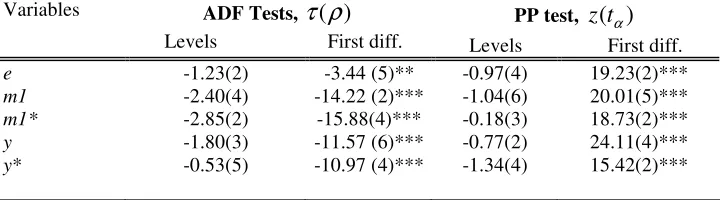
and first differences are presented in table 1. The results show that we fail to reject the

However, the null is rejected for the first difference. This implies that the series are

integrated of order one I(1).

<TABLE 1 ABOUT HERE>

3.2 Cointegration Analysis

If a system (set) of the series is found to be cointegrated, they are linked together

through a long-run relationship that prevents them from diverging. In a cointegration test

involving three or more variables, we apply the maximum likelihood method suggested

by Johansen (1988, 1991) and Johansen and Juselius (1990). It is based on a vector

error-correction model of the form:

1

1 k

X_t X_{t k i} X_{t i} e t i

µ

−

∆ = + Π ₋ + Γ ∆ ₋ +

= (15)

where Xt is a (m x 1) vector of exchange rates. The parameter matrix Π contains

information as to whether there is a long-run relationship among variables. The rank of

Π equals the number of cointegration vectors. If the rank of the matrix Π is zero, the

system reduces to a standard vector autoregression model, implying no long-run

relationship among variables. If Π has a full rank, then all the variables are stationary.

Cointegration is implied when the rank of Π is intermediate. That is, if 0 < rank(Π) < m,

there exists r cointegrating vectors which make the linear combination of Xt stationary.

To test the rank of Π, Johansen and Juselius make use of maximum eigenvalue and trace

3.3 Estimated Results

The existence of long-run cointegrating vectors was tested using Johansen’s

Maximum Likelihood Procedure (see, for example, Johansen 1988; Johansen and Juselius

1990). The Johansen cointegration test is sensitive to the choice of lag length. To

determine the most appropriate lag length, the Akaike Information Criteria (AIC) was

used. In addition, the residuals in the Johansen VAR were checked for misspecification.

To capture any serial correlation, extra lags were added until this was removed.

According to Gonzalo (1994), the costs of over-parameterization in terms of efficiency

loss is marginal, but this is not the case in the event of under-parameterization. Further,

when testing for cointegration, the question of whether a trend should be included in the

long-run relationship arises. As Hendry and Doornik (1994) pointed out, the trend is

restricted to the cointegrating space, to take into account long-run exogenous growth

which is not already included in the model.

<TABLE 2 ABOUT HERE>

The results for the cointegration test on the unrestricted model are presented in

table 2. Based on AIC, a lag length of 6 was chosen. The maximum eigenvalue test

statistic reveals one significant cointegrating relationship, whereas the trace statistic

suggests there are two cointegrating vectors. This indicates the presence of one

cointegrating relationship based on the evidence of the stronger maximum eigenvalue test

(Johansen and Juselius, 1990). The results for the normalized equation are reported in

<TABLE 3 ABOUT HERE>

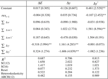
The results of the unrestricted error correction model are included in table 4. The

residuals from the cointegrating vector, with one lag, act as the error correction term.

This term captures the disequilibrium adjustment of each variable towards its long-run

value. The coefficient on the error correction terms in each individual equation

represents the speed of adjustment of this variable back to its long-run value. A

significant error correction term implies long-run causality from the explanatory variables

to the dependent variables (Granger, 1988).6

<TABLE 4 ABOUT HERE>

In Table 4 the first statistic represents the sum of the coefficients on the lagged

differences of the variables. The second statistic (in the brackets) 7 is a chi-square statistic

indicating the significance levels of the sum of the coefficients. This can be interpreted as

capturing the short-run dynamics in the model and indicates short-run causality between

the variables.

For the exchange rate equation, there is evidence of short-run causality from the

Kenyan and U.S. money supply to the exchange rate, as well as short-run causality from

Kenyan income to the exchange rate. For money supply equations there is less evidence

of short-run causality, particularly running from the exchange rate to money supply. This

indicates that causality predominantly runs from money supply to the exchange rates. The

explanation for this phenomenon is observed when one takes into consideration the

supply will lead to a decline in the interest rate. This will result in depreciation of the

KSH due to capital flight.

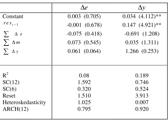
The error correction results for the restricted model are included in Table 5. Once

again the error correction term is only significant for the money supply equation. As with

the unrestricted model, there is some evidence of short-run causality from money supply

to the exchange rate, but no evidence of causality in the other direction. The main feature

of the money supply equation is the strong causality to the exchange rate differential from

previous differentials. Both equations are well specified, although the explanatory power

is low.

<TABLE 5 ABOUT HERE>

Finally, a further test of the monetary approach to exchange rate dynamics model

is how well it forecasts out of sample. The exchange rate equation was estimated from

June 1990 to December 2004, and 2005 was used for forecasting. Following the lead of

other studies in the literature, the forecasting performance is compared to a random walk.

In addition, both the restricted and unrestricted models are compared to the forecasting

performance of the Frankel Real Interest Differential model.8 The root-mean-square

error (RMSE) statistics from all four models are compared in Table 6. Ironically the

worst performer is the unrestricted model, while the best is the restricted model. The

Frankel model fails to beat the random walk over short time horizons, but over longer

time horizons is the second best forecaster of the exchange rate. In addition, the

significance of each of the measures of forecast accuracy is tested using the Diebold and

forecast minus the benchmark random walk forecast) is regressed on a constant. Only the

restricted model and Frankel model produce forecasts that are significantly different from

the benchmark random walk model.

<TABLE 6 ABOUT HERE>

4.0 CONCLUSION

This paper has examined the relationship between the money supply, income

(output) and exchange rate by applying the monetary model of exchange rate

determination. The results indicate that in equilibrium, this version of the monetary

model produces a cointegrating vector, in which the money supply variable is the most

significant determinant of the exchange rate in Kenya. The dynamic results produce well

specified error correction models. However there is very little evidence that exchange

rates have a significant effect on money supply (i.e. reverse causality).

These findings suggest that, in general, models of the equilibrium exchange rate

determination must be extended to encompass both internal and external factors. This can

help in monetary policy coordination, for instance, to avert a financial crisis triggered by

speculative attack on a small open economy. Finally, the restrictions implicit in the

monetary model of the exchange rate appear to hold over the post exchange rate float

period. This finding is supported by the forecasting performance of the models, in which

the restricted model outperforms all the alternatives over short and long time horizons.

These results add to other recent studies which portray the monetary models generally in

FOOTNOTE

1

Chrystal and Macdonald (1995) find evidence of a valid long-run relationship using divisia money while Choudhry and Lawler (1997) find evidence of a long-run

relationship for the restricted monetary model using Canadian/US data for the 1950s float.

2

This possibility was pointed out by Young (1992).

3

An advantage of using the FLME, is that it produces a model in which stock prices are the explanatory variables along with income and money. If the conventional monetary model, with static expectations or Frankel real interest rate model had been used, both long and short interest rates would have been incorporated into the model, which could have produced problems of collinearity between the interest rates and stock price returns in the ECMs. In general, the conventional FLME (without stock prices) is not widely used because it usually fails to produce evidence of a valid long-run equilibrium relationship and it is not a good predictor of the exchange rate.

4

Testing for cointegration between the exchange rate and forcing variables is also a test for the presence of bubbles in the exchange rate. If cointegration is found and certain restrictions prove to hold, then the speculative bubble hypothesis is rejected. However, this line of investigation is beyond the scope of this paper. Assuming UIP means the interest rate differential equals the expected rate of depreciation. In the absence of arbitrary bubbles, the rate of expected appreciation is some function of expected movements in fundamentals, and so equation (8) must be true.

5

For values of λ close to unity, adjustment is very rapid, with the disequilibrium being totally eliminated within one period of time. For 0<λ<1 the dynamic adjustment path will be monotonically convergent.

6

Given that the Johansen maximum Likelihood procedure is essentially a vector autoregression (VAR) based technique, it is more appropriate to produce the complete ECM rather than a parsimonious specification , in which the non-significant lags are omitted.

7

See notes in Table 4 for details.

8

REFERENCES

Campbell, J.Y., and Shiller, R.J. 1987. “Cointegration and Tests of Present Value Models,” Journal of Political Economy, 95, 1062-88.

Choudhry and Lawler. 1997. “The Monetary Model of Exchange Rates: Evidence from the Canadian Float of the 1950's,” Journal of Macroeconomics, 19, 349-362.

Culver S.E., and Papell, D. 1999. “Long-Run Purchasing Power Parity with Short-run Data: Evidence with a Null Hypothesis of Stationarity,” Journal of International Money and Finance, 18 (5), 751-768

Dickey, D. A. and W. A. Fuller. 1981. “Likelihood Ratio Statistics for Autoregressive Time Series with a Unit Root,” Econometrica 49, 1057-1072.

Dickey, D.A. and W. Fuller. 1979. “Distribution of Estimators for Autoregressive Time Series with a Unit Root,” Journal of the American Statistical Association, 74, 427-431.

Diebold, F.X. and R.S. Mariano. 1995. “Comparing Predictive Accuracy,” Journal of Business and Economic Statistics, 13, 253-263.

Dornbusch, R. 1976. “Expectations and Exchange Rate Dynamics,” Journal of Political Economy, Vol. 84, pp. 1161-76.

Engle, R. F. 1982. "Autoregressive conditional heteroscedasticity with estimates of the variance of United Kingdom inflation", Econometrica, 50, 987-1006.

Gonzalo, J. 1994. “Five alternative methods of estimating long-run equilibrium relationships, Journal of Econometrics, 60, 203-233.

Granger, C. 1988. “Causality, Cointegration, and Control, Journal of Economic Dynamics and Control,” 12, 511-59.

Hendry, D.F. and Doornik, J.A. 1994. “Modelling Linear Dynamic Econometric Systems,” Scottish Journal of Political Economy, 41, 1-33.

Johansen, S. 1988. “Statistical Analysis of Cointegration Vectors”, Journal of Economic Dynamics and Control, 12, 231-254.

Johansen, S. and K. Juselius. 1990. “Maximum Likelihood Estimation And Inference on Cointegration with Applications to the Demand for Money,” Oxford Bulletin of Economics and Statistics, 52, 169-210.

K.A. Chrystal, R. MacDonald. 1995. “Exchange Rates, Financial Innovation and Divisia Money: the Sterling/Dollar Rate 1972-1990,” Journal of International Money and Finance, 14 (4) (1995) pp. 493-513.

MacDonald, D. and M.P. Taylor (1989) Foreign Exchange Market Efficiency And Cointegration: Some Evidence From The Recent Float, Economic Letters 29 (1), pp. 63-68.

McNown, R., and Wallace, M., 1989. “Cointegration Tests for Long Run Equilibrium in the Monetary exchange Rate Model,” Economics Letter, 31, 263-67.

Meese, R. 1986. “Testing for Bubbles in Exchange Markets: A Case of Sparkling Rates,” Journal of Political Economy, 94(2), 345-373.

Philips, P.C.B., and Perron, P. (1988) Testing for a Unit Root in Time Series Regressions,” Biometrika, 75, 335-346.

Young, A. 1992. “A Tale of Two Cities: Factor Accumulation and Technical Change in Hong Kong and Singapore,” NBER Macroeconomics Annual, 13-53.

Table 1: Unit Root Tests

Variables ADF Tests, τ ρ( )

Levels First diff.

PP test, z t( )_α

Levels First diff.

e -1.23(2) -3.44 (5)** -0.97(4) 19.23(2)***

m1 -2.40(4) -14.22 (2)*** -1.04(6) 20.01(5)***

m1* -2.85(2) -15.88(4)*** -0.18(3) 18.73(2)***

y -1.80(3) -11.57 (6)*** -0.77(2) 24.11(4)***

y* -0.53(5) -10.97 (4)*** -1.34(4) 15.42(2)***

Notes: The critical ADF and PP values are taken from Dickey and Fuller (1981) and Philips and Perron (1988) respectively. The regressions were done with a constant term only and the lag length is based on AIC are in parentheses, which are selected to eliminate serial correlations. Seasonal dummies were included to control for seasonal unit roots (not reported here, but available from the authors upon request). *** and ** indicate 1% and 5% significance levels, respectively.

Table 2-Johansen Maximum Likelihood Test for Cointegration of the Unrestricted and Restricted Models

Unrestricted Model Restricted Model

Vectors Trace Test Eigenvalue Test Trace Test Eigenvalue Test

r =0 1 ≤ r 2 ≤ r 3 ≤ r 4 ≤ r 5 ≤ r 6 ≤ r 177.92** 127.41** 84.09 53.63 31.11 14.75 4.96 50.52** 43.31 30.47 22.51 16.36 9.80 4.96 78.00** 31.98 15.07 5.32 46.01** 16.92 9.75 5.32

Table 3- Normalized Equations of the Cointegrating Vectors

Notes: The significance of the coefficients were tested using the LM statistic which tests the restriction that the coefficient is equal to zero. (χ_{0 5}2_. ( )_{1 =3841}. )_.

** indicates significance at the 5% level.

Table 4-Error Correction Model Results for the Unrestricted Model

∆E ∆y *

y

∆

Constant

res_t−1

0.017 [0.305] -0.004 [0.328] -0.126 [0.607] 0.035 [0.736] 0.481 [2.529]** -0.107 [2.452]** ∆e 1 m ∆ 0.096 (0.619) 0.084 (0.343) -0.090 (1.900) 1.022 (2.774) -0.031 (0.938) 1.581 (8.594)** * 1 m ∆ y ∆ 0.187 (0.645) -0.318 (3.994)** -0.478 (0.030) 1.161 (4.283)** 1.504 (0.191) -0.001 (0.073) * y

∆ 0.324 (1.274) -1.606 (4.839)** -1.082 (1.236)

R2 SC(12) SC(6) Reset Heteroskedasticity ARCH(12) 0.687 1.658 1.417 0.077 0.522 0.482 0.706 2.022 1.019 0.232 0.204 0.155 0.813 0.827 1.021 1.573 0.122 0.989

Notes: res denotes the error correction term; R2 is the coefficient of determination; DW is

the Durbin-Watson statistic; SC(i) are the ith order tests for serial correlation; ARCH(i) is Engle’s (1982) test for the ith autoregressive conditional heteroskedasticity. These test statistics follow the F-distribution. Critical values are: F(6,222) = 2.14, F(12,216) = 1.80, F(1,227) = 3.89. The values in brackets represent t-statistics. The values in parentheses represent Wald statistics, which follow a chi-square distribution with critical value 3.842. All equations include seasonal dummies.

** indicates significance at the 5% level.

Unrestricted Model Restricted model

Table 5- Error Correction Model for the Restricted Model

e

∆ ∆y

Constant

r e st−1

0.003 (0.705) -0.001 (0.678)

0.034 (4.112)** 0.147 (4.921)**

e ∆

m ∆

-0.075 (0.418) 0.073 (0.545)

-0.691 (1.208) 0.035 (1.311)

y

∆ 0.061 (0.064) 1.266 (0.253)

R2 SC(12) SC(6) Reset Heteroskedasticity ARCH(12) 0.08 1.592 0.320 1.510 1.025 0.795 0.189 0.746 0.524 3.913 0.007 0.920

Notes: See Table 4

Table 6- RMSE Statistics for Forecasts using the Competing models (ECM and Random Walk)

Models 3 Months 6 Months 9 Months 12 Months

Random Walk Unrestricted Model Restricted Model Frankel Model 0.010 0.013 0.009 0.011 0.017 0.017 0.016** 0.016** 0.017 0.018 0.016** 0.016** 0.016 0.017 0.015** 0.015**