A Novel Feature Subset Selection Algorithm for
Software Defect Prediction
Reena P
Department of Computer science and Engineering SCT College of Engineering
Trivandrum, India
Binu Rajan
Department of Computer science and Engineering SCT College of Engineering
Trivandrum, India
ABSTRACT
Feature subset selection is the process of choosing a subset of good features with respect to the target concept. A clustering based feature subset selection algorithm has been applied over software defect prediction data sets. Software defect prediction domain has been chosen due to the growing importance of maintaining high reliability and high quality for any software being developed. A software quality prediction model is built using software metrics and defect data collected from a previously developed system release or similar software projects. Upon validation of such a model, it could be used for predicting the fault-proneness of program modules that are currently under development. The proposed clustering based algorithm for feature selection uses minimum spanning tree based method to cluster features. And then the algorithm is applied over four different data sets and its impact is analyzed.
General Terms
Relevant features, Redundant Features, Minimum spanning tree, Tree partition, graph based clustering, Software defect prediction, Naïve Bayes classifier, Decision tree classifier
1.
INTRODUCTION
Feature subset selection is the process of choosing a subset of good features with respect to the target concepts. It is an effective way for reducing dimensionality, removing irrelevant data, increasing learning accuracy, and improving result comprehensibility. Many feature subset selection methods have been proposed and studied for machine learning applications.
Software Defect Prediction has been an area of growing importance. It is always required to maintain high reliability and high quality for any software being developed. A software quality prediction model is built using software metrics and defect data collected from a previously developed system release or similar software project. Upon validation of such a model, it could be used for predicting the fault-proneness of program modules that are currently under development. A low quality or fault prone prediction can justify the application of available quality improvement resources to those programs. In contrast, a non fault prone prediction can justify non-application of the limited resources to these already high-quality programs. And finally high software reliability and quality are maintained with an effective use of the available resources. A feature extraction algorithm based on graph
for defect prediction purpose and its impact on different data sets are analyzed in this paper.
1.1
Data Set
The software data sets provided by the NASA IV&V Metrics Data Program – Metric Data Repository are being used for majority of the experiments related with software engineering. The data repository contains software metrics as attributes in the data sets and also an indication of whether a particular set of data is defective or non-defective. All the datacontained in the repository are collected and validated by the Metrics Data Program.
Some of the product metrics that are included in the data set are, Halstead Content, Halstead Difficulty, Halstead Effort, Halstead Error Estimate, Halstead Length, Halstead Level, Halstead Programming Time and Halstead Volume, Cyclomatic Complexity and Design Complexity, Lines of Total Code, LOC Blank, Branch Count, LOC Comments, Number of Operands, Number of Unique Operands and Number of Unique Operators, and lastly Defect Metrics; Error Count, Error Density, Number of Defects (with severity and priority information).
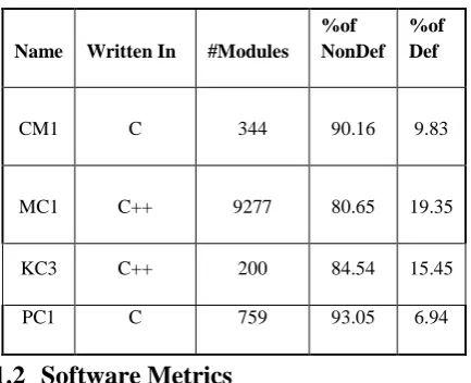
[image:1.595.319.536.538.714.2]The details about datasets used for assessing the proposed feature extraction algorithm are given below:
Table 1. Defect prediction Datasets
Name Written In #Modules %of NonDef
%of Def
CM1 C 344 90.16 9.83
MC1 C++ 9277 80.65 19.35
KC3 C++ 200 84.54 15.45
PC1 C 759 93.05 6.94
1.2
Software Metrics
are listed below. Metrics that does not come under these three categories are given under others.
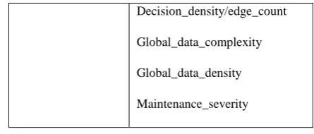
Table 2. Software Metrics
Metrics Type Definition
McCabe
Complexity metrics
Cyclomatic complexity
Design complexity
Essential complexity
LOC
Loc_total
LOC_blank
LOC_code_and_comment
LOC_comments
LOC_executable
Number_of_lines
Operator Number_of_operands
Number of _operators
Number_unique operands
Number_unique operators
Halstead metrics
Length
Volume
Level
Difficulty
Content
Error Estimate
Programming time
Effort
Others
Branch count
Call_pairs
Condition_count
Decision_count
Decision_density/edge_count
Global_data_complexity
Global_data_density
Maintenance_severity
2.
RELATED WORK
Feature subset selection is the process of identifying and removing irrelevant and redundant features as much as possible. Number of methods has been proposed in the past for feature selection. Some of them efficiently removes irrelevant attributes but fails to eliminate redundant attributes whereas some others eliminate redundant attributes and fails to remove redundant features.
One of the traditional methods that focused on retaining the relevant features is Relief [1]. This feature set estimator evaluates each feature individually. A relevance value is assigned to each feature and features with relevance value greater than a threshold are selected. Original relief handled only Boolean problems but extensions of relief such as Relief-f and RrelieRelief-f-Relief-f works on classiRelief-fication problems too. The extensions of relief differ from original relief in the chosen neighbors and evaluation function. The drawback of relief is that it cannot determine redundant attributes or any other redundant rules.
Mutual Information theory can also be used for selecting features especially in neural network learning [2]. Here mutual information criterion is used to evaluate a set of candidate features and then an informative subset is selected which can be given as input data for neural network classifier. Mutual information based feature selection method are useful for complex classification problems where methods based on linear relations like correlation are prone to failure. Mutual information measures arbitrary dependencies between random variables.
FOCUS-II [3] is an algorithm for picking up the relevant features from a set of features. It implements MIN-FEATURES bias, which prefers consistent hypothesis definable over as few features as possible. It is faster than FOCUS algorithm. Mutual Information greedy, simple greedy and weighted greedy algorithms also apply efficient heuristics for approximating the MIN-FEATURES bias. The paper focuses on the methods for reducing the computational costs involved in implementing the MIN-FEATURES bias. When weighted greedy sample algorithm is used for preprocessing the training sample, then decision tree classifier gives a better result.
3.
PROPOSED WORK
A number of methods and techniques have been already proposed and implemented in the field of software defect prediction. The algorithm used for feature selection plays a crucial role in every defect prediction problem. This paper focuses on a two level clustering based feature selection algorithm which can be used with any software defect prediction framework. The proposed algorithm is applied over different software defect prediction data sets and their performance discrepancies are analyzed.
A high level design framework of the proposed system is given below:
Figure 1: High Level Design Framework
3.1
Two Level Feature Subset Selection
Algorithm
Two level feature subset selection algorithms effectively deal with redundant and irrelevant attributes. The first level of algorithm removes the redundant attributes and irrelevant attributes are eliminated in the last phase. Such a two level clustering based preprocessing algorithm has been tested over different software defect prediction data sets and the procedure is explained in detail below.
3.2
Removal of Irrelevant Attributes
Those attributes in a data set that have a strong correlation with the target concept is termed as a relevant attribute. All those attributes that are not relevant are called irrelevant attributes. Relevant attributes are always necessary for the
correlation based approach is used for choosing the relevant features.
Pearson’s correlation coefficient can be computed using the formula given below:
Here Xi and Yi refer to a pair of sample data, X and Y refer to any two attributes of data set. Pearson’s correlation value for each attribute with the target attribute is to be calculated and this is taken as T-Relevance value of each feature. The above given formula applies when both the given attributes are continuous. For defect prediction data sets, the target attribute is discrete and other attributes are continuous. The formula given below is used for calculating the T-Relevance between continuous and discrete attributes.
Where ‘r’ refers to Pearson’s Correlation (T-Relevance) value, Xbi is a binary attribute that takes value 1 when X has value xi and 0 otherwise.
Here T-Relevance value is then compared with a predetermined threshold value. The threshold value is determined based on the formula given below:
Threshold Value = T-Relevance of √mth ranked value attribute where m is the total number of attributes in the chosen data set.
If the calculated T-Relevance is less than predetermined threshold value, that indicates the attribute is irrelevant and is removed from the attribute subset. Hence the subset is reduced to only relevant features.
3.3
Minimum Spanning Tree Construction
For a data set with features = { 1, 2,..., } and class , the T-Relevance also called Symmetric Uncertainty ( , ) value for each feature (1 ≤ ≤ ) is computed in the first step. The attributes whose ( , ) values are greater than a predefined threshold encompass the target-relevant feature subset ′ = { ′1, ′2,..., ′ } ( ≤ ).In this phase F-Correlation ( ′ , ′ ) value for each attribute is calculated. Pearson’s Correlation formula which has already been described in the first phase is used for this purpose. Here all the attributes are continuous valued and therefore normal Pearson’s Correlation formula is used.
After calculating the F-Correlation ( ′ , ′ ) value for each pair of features ′ and ′ ( ′ , ′ ∈ ′ ∧ != ). Then, a weighted complete graph G=(V,E) is constructed using features ′ and ′ as vertices and ( ′ , ′ )( != ) as the weight of the edge between vertices ′ and ′ . ( ′ , ′ )= ( ′j, ′i), and therefore G is an undirected graph. The weighted complete graph G shows correlations among all the target-relevant features. Now graph has vertices and ( −1)/2 edges. For high dimensional data, it is heavily intense and the edges with different weights are strongly interwoven. Moreover, the decomposition of complete graph is NP-hard. Thus for graph , a Minimum Spanning Tree
ki
Y X i
XY
P
X
x
r
b ir
1
)
(
LOAD CHOSEN DEFECT PREDICTION DATA SETS
IRRELEVANT FEATURE REMOVAL
MINIMUM SPANNING TREE CONSTRUCTION
TREE PARTITION AND REPRESENTATIVE FEATURE
SELECTION
SELECTED FEATURE SUBSET
CLASSIFIERS FOR DEFECT PREDICTION
Prim’s algorithm is used for constructing the minimum spanning tree.
3.4
Tree Partitioning and Elimination of
Redundant Features
The minimum spanning tree is constructed in the second step. Now in the third step, partitioning of the tree is to be done based on graph clustering. In the minimum spanning tree, each vertex is assigned its value as its T-Relevance (SU( ′ , )) value with the class attribute. In this step, those edges are removed where = {( ′ , ′ ) ∣ ( ′ , ′ ∈ ′ ∧ , ∈[1, ] ∧ != }, that is whose weights are smaller than both of the T-Relevance ( ′ , ) and ( ′ , ), from the MST. Whenever an edge is deleted, two disconnected trees T1 and T2 are obtained. This technique is recursively applied over each disconnected trees and finally a set of clusters is obtained. Each cluster consists of one or more number of vertices. When a cluster has more than one attribute, by the property of redundant features it indicates that the cluster has redundant features. So a single representative features from each cluster need to be selected for final subset. For this, the vertex with highest T-Relevance value is chosen from each cluster and is added to the final subset. Thus the final subset of features is obtained in the third step.
3.5
Performance Report Generation
To evaluate the performance of the implemented feature extraction algorithm, classifiers need to be implemented. Two classifiers namely, decision tree classifier and Naïve Bayes classifiers are implemented. The proposed feature extraction algorithm is applied over four defect prediction data sets namely CM1, KC3, MC1 and PC1. And then the data before preprocessing and after preprocessing are separately given to the two above said classifiers.
4.
RESULTS
Four matrices are considered for performance comparison of the implemented feature extraction algorithm over four different data sets namely Proportion of selected features, Time taken for classification, Classification accuracy and Precision. Each of them is shown in separate tables given below.
Table 3. Proportion of Selected Features Among Different Data Sets.
Data Set
Total Features
Features After Extraction
Proportion Of Selected Features
Number of Instances
CM1 36 28 0.77778 344
KC3 38 19 0.5 200
MC1 37 11 0.29729 9277
PC1 36 23 0.63889 759
[image:4.595.313.547.424.570.2]The proportion of selected features is maximum for CM1 data set and minimum for MC1 data set. This has impact on the classification accuracy and precision.
Table 3. Classification Accuracy Before And After Preprocessing.
DATA
ACCURACY
NAÏVE BAYES DECISION TREE BEFORE AFTER BEFORE AFTER CM1 .82848 .82558 0.95930 0.95639
KC3 0.8 0.815 0.915 0.92
[image:4.595.51.294.543.694.2]MC1 0.93716 0.93747 0.99719 0.99698 PC1 0.88669 0.88274 0.96969 0.96179
Table 4. Classification Precision Before And After Preprocessing.
DATA
PRECISION
NAÏVE BAYES DECISION TREE BEFORE AFTER BEFORE AFTER
CM1 0.90909 0.90333 0.96753 0.9644 KC3 0.8647 0.86705 0.93491 0.94578 MC1 0.99689 0.99689 0.99794 0.99794 PC1 0.94348 0.93813 0.98009 0.97582
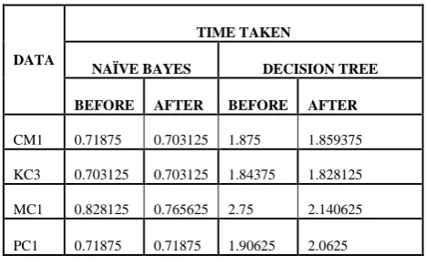
Table 4. Time taken for Classification Before And After Preprocessing.
DATA
TIME TAKEN
NAÏVE BAYES DECISION TREE
BEFORE AFTER BEFORE AFTER
CM1 0.71875 0.703125 1.875 1.859375
KC3 0.703125 0.703125 1.84375 1.828125
MC1 0.828125 0.765625 2.75 2.140625
PC1 0.71875 0.71875 1.90625 2.0625
5.
CONCLUSION
more, there is more reduction in the time taken for classification. So if the feature extraction algorithm is applied over a high dimensional data, high performance can be guaranteed since there will be more reduction in time which can compensated for slight loss in classification accuracy or precision. Hence an improved software defect predictor can be built that would not compromise on the quality but would reduce the overall cost of developing any software.
As a future work the implemented feature extraction algorithm can be tested over other available data sets in the same domain, it can be tested over data sets in other domains too. In addition, additional classifiers can be applied over data sets in the same domain which would give better results than the already implemented classifiers.
6.
REFERENCES
[1] Antonio Arauzo-Azofra, Jose Manuel Benitez and Juan Luis Castro, A Feature Set Measure Based On Relief, RASC2004.
[2] Roberto Battiti, Using Mutual Information For Selecting Features In Supervised Neural Net Learning, IEEE Transactions on Neural Networks 1994, VOL 5, NO 4, July 1994.
[3] Hussein Almuallim, Thomas G Dieterich , Efficient Algorithms For Identifying Relevant Features 1991. [4] George Forman, An Extensive Empirical Study Of
Feature Selection Metrics For Text Classification,
Journal of Machine Learning Research 3 (2003) 1289-1305.
[5] M Scherf, W Brauer, Improving RBF Networks By The Feature Selection Approach EUBAFES.
[6] Guyon I. and Elisseeff A., An introduction to variable and feature selection, Journal of Machine Learning Research, 3, pp 1157-1182, 2003.
[7] Mitchell T.M., Generalization as Search, Artificial Intelligence, 18(2), pp 203-226, 1982.
[8] Dash M. and Liu H., Feature Selection for Classification, Intelligent Data Analysis, 1(3), pp 131-156, 1997. [9] Langley P., Selection of relevant features in machine
learning, In Proceedings of the AAAI.
[10] Qinbao Song, Jingjie Ni and Guangtao Wang , A Fast Clustering-Based Feature Subset Selection Algorithm for High Dimensional Data, IEEE Transactions On Knowledge And Data Engineering Vol:25 No:1 Year 2013.
[11] Tim Menzies, Jeremy Greenwald, and Art Frank “Data Mining Static Code Attributes to Learn Defect Predictors”, IEEE Transactions On Software Engineering, Vol. 33, No. 1, January 2007.