R E S E A R C H
Open Access
A new generalization of generalized
half-normal distribution: properties and
regression models
Emrah Altun
1*, Haitham M. Yousof
2and G.G. Hamedani
3*Correspondence: [email protected] 1Department of Statistics, Bartin
University, Bartin 74100, Turkey Full list of author information is available at the end of the article
Abstract
In this paper, a new extension of the generalized half-normal distribution is introduced and studied. We assess the performance of the maximum likelihood estimators of the parameters of the new distribution via simulation study. The flexibility of the new model is illustrated by means of four real data sets. A new log-location regression model based on the new distribution is also introduced and studied. It is shown that the new log-location regression model can be useful in the analysis of survival data and provides more realistic fits than other competitive regression models.
Keywords: Regression, Residuals, Simulation
AMS 2010 Subject Classification: 60E05, 62J05
Introduction
The generalized half-normal (GHN) distribution has been widely modified and stud-ied in recent years and various authors developed new generalizations of it. Following an idea due to Eugene et al. (2002), Pescim et al. (2017) introduced the beta general-ized half-Normal (BGHN) distribution with applications to myelogenous leukemia data. Cordeiro et al. (2012) defined the Kumaraswamy generalized half-normal (KwGHN) dis-tribution for censored data. More recently, Cordeiro et al. (2013) studied some of the mathematical properties of the BGHN distribution proposed by Pescim et al. (2010b). Pescim et al. (2013) proposed the log-linear regression model based on the BGHN dis-tribution, while Ramires et al. (2013) defined the beta generalized half-normal geometric (BGHNG) distribution in order to achieve wider diversity among the density and failure rate functions.
The GHN density function (Cooray and Ananda2008) with shape parameterλ >0 and scale parameterθ >0 is given (forx>0) by
g(x;λ,θ)=
2
π λ
x x θ
λ exp
−1
2 x
θ 2λ
, (1)
and its cumulative distribution function (cdf ) depends on the error function
G(x;λ,θ)=2x
θ λ
−1=erf
x
θ λ √
2
, (2)
where
(x)= 1 2
1+erf
x √ 2 and
erf(x)= √2 π
x
0
exp(−t2)dt.
Thenth moment of the random variableXwith cdf (2) is
E(Xn)=
n+λ 2λ
2nλ π θ−n ,
where (.) is the gamma function. The HN distribution is a sub-model of GHN when
λ=1.
The goal of this paper is to propose the first generalization of the generalized half-normal distribution using the Zografos–Balakrishnan Odd Log-Logistic-G (“ZBOLL-G” for short) family of distributions. For an arbitrary baseline cdfG(x), Cordeiro et al. (2015) proposed the probability density function (pdf )f(x)and the cdfF(x)of the ZBOLL-G family of distributions with two additional shape parametersβ >0 andα >0 as
f(x;β,α,ξ)= α
(β)
g(x;ξ)Gα−1(x;ξ)G¯α−1(x;ξ)
Gα(x;ξ)+ ¯Gα(x;ξ)2
−log G¯ α(x;ξ)
Gα(x;ξ)+ ¯Gα(x;ξ) β−1
(3)
and
F(x;β,α,ξ)= 1
(β)γ
β,−log
1− G
α(x;ξ)
Gα(x;ξ)+ ¯Gα(x;ξ)
, x∈ , (4)
whereξ denotes the parameter vector of the baseline distribution. We use Eqs. (1), (2) and (3) to obtain the four-parameter ZBOLLGHN pdf (forx>0)
f(x)= α 2 π λ x x θ λ exp −1 2 x θ 2λ
2xθλ
−1 α−1
2−2xθλ α−1
(β)2θxλ−1α+2−2xθλα2
× ⎡ ⎢ ⎣−log
⎛ ⎜ ⎝
2−2xθλ α
2θxλ−1α+2−2xθλα ⎞ ⎟ ⎠ ⎤ ⎥ ⎦ β−1 , (5)
whereα > 0,β > 0,λ > 0 are shape parameters andθ is the scale parameter. The corresponding cdf is given by
F(x)= 1 (β)γ
⎡ ⎢ ⎣β,−log
⎛ ⎜ ⎝1−
2θxλ−1α
2θxλ
−1 α
+2−2xθλ α ⎞ ⎟ ⎠ ⎤ ⎥
⎦, x≥0,
(6)
where γ (β,z) = ∞ # z
tβ−1exp(−t)dt denotes the complementary incomplete gamma
Table 1Submodels of ZBOLL-GHN distribution
Distribution β α λ θ Author
Gamma-GHN β 1 λ θ New
Gamma-HN β 1 1 θ New
OLL-GHN 1 α λ θ Cordeiro et al. (2016b)
OLL-HN 1 α 1 θ Cordeiro et al. (2016b)
GHN 1 1 λ θ Cooray and Ananda (2008)
HN 1 1 1 θ Cooray and Ananda (2008)
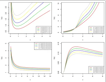
We investigate the possible hazard rate function (hrf ) and pdf shapes of ZBOLL-GHN distribution. Figure1displays the pdf shapes of ZBOLL-GHN distribution. Based on the Fig.1, ZBOLL-GHN pdf has the following shapes: left-skewed, right-skewed, symmetric and bimodal. Figure2displays the hrf shapes of ZBOLL-GHN distribution. From Fig.2, we conclude that the ZBOLL-GHN hrf has the following shapes: increasing, decreasing, upside-down and bathtub.
Following Cordeiro et al. (2016a), equation (6) can be expressed as
F(x)= ∞ $
w=0
bww(x;λ,θ),
where
bw= 1
(β) ∞ $
i,k=0
k $
j=0
(−1)i+j+k
β+i−ji!pj,kaw(β,α,i,k)
k−β−i k
k
j
andw(x;λ,θ) = [G(x;λ,θ)]w denotes the cdf of the exp-GHN distribution with the power parameterw. The pdf (5) reduces to
f(x)= ∞ $
w=0
bw+1πw+1(x;λ,θ), (7)
whereπw+1(x;λ,θ)=(w+1)g(x;λ,θ)[G(x;λ,θ)]wdenotes the pdf of the exp-GHN
dis-tribution with the power parameterw+1. For the definitions ofpj,k andaw(β,α,i,k), please see Cordeiro et al. (2016a). Equation (7) reveals that the density function ofXis a linear combination of the exp-GHN densities. Thus, some of the structural properties of the ZBOLL-GHN distribution such as ordinary and incomplete moments and generating function can be obtained from well-established properties of the exp-GHN distribution.
Fig. 2The hrf plots of ZBOLL-GHN distribution for selected parameter values
We are motivated to introduce the ZBOLL-GHN distribution since it contains a number of aforementioned known lifetime models as illustrated in Table 1. The new distribution exhibits increasing, decreasing, upside-down as well as bathtub hazard rates as illustrated in Fig.2. It is shown that the new distribution can be viewed as a mixture of the two-parameter GHN model. It can also be viewed as a suitable model for fitting the left-skewed, right-skewed, symmetric and bimodal data. The ZBOLL-GHN distribu-tion outperforms several of the well-known lifetime distribudistribu-tions with respect to four real data applications as illustrated in “Applications” section. The new log-location regression model based on the ZBOLL-GHN distribution provides better fits than log BGHN, log GHN and log-Weibull models for volatage data set. Based on the residual analysis (mar-tingale and modified deviance residuals) for the new log-location regression model (log ZBOLL-GHN), we conclude that none of the observed values appear as possible outliers. Thus, it is clear that the fitted model is appropriate for the voltage data set.
The rest of the paper is organized as follows. In “Estimation” section, the maximum likelihood method is used to estimate the model parameters. The performance of maxi-mum likelihood estimators of the model parameters are investigated by means of a Monte Carlo simulation study whennis finite. A new log-location regression model as well as residual analysis are presented in “A new log-location regression model” section. Four applications to real data sets illustrate empirically the importance of the new model in “Applications” section. Finally, a summary is provided in “Summary” section.
Estimation
()=log(α)+log %
2
π &
+log(λ)−log(x)+λlogxθ−1− 1 2
xθ−12λ
+(α−1)log(w−1)+(α−1)log(2−w)−log [ (β)]
−2 log(w−1)α+(2−w)α+(β−1)log
−log
(
2−w)α (w−1)α+(2−w)α
.
The components of the unit score vectorU =U()=(∂β/∂,∂α/∂,∂λ/∂,∂θ/∂)T are available if needed. For a random samplex = (x1, ...,xn)T of sizenfromX, the total log-likelihood is
n()= n $
i=0 (i)(),
where(i)()is the log-likelihood for the ithobservation. The total score function is
Un= n $
i=0 U(i),
whereU(i) has the form given before. Maximization of ()(orn()) can be easely performed using well-established routines such as thenlmoroptimin the R statistical package. Setting these equations equal to zero,U()= 0, and solving them simultane-ously gives the MLE'of. These equations cannot be solved analytically and statistical software can be used to evaluate them numerically using iterative techniques such as the Newton-Raphson algorithm.
The parameter estimation procedure of ZBOLL-GHN model can be summarized as follows:
• Theoptimfunction of R software is used to minimize the minus log-likelihood function of GHN model by means of the Nelder-Mead (NM) optimization method. There is no need to provide the derivatives of the objective function for NM method.
• The estimated parameters of GHN distribution are used as initial values of the ZBOLL-GHN model. The initial values of the additional parametersαandβare chosen as 1. Note that the ZBOLL-GHN model reduces to GHN model when the
parametersα=β=1. Then, the parameter estimation of ZBOLL-GHN model are
obtained with theoptimfunction as given in the first step.
• The inverse of estimated Hessian matrix is used to obtain the corresponding standard errors.
Simulation study
(
Bias(n)= 1 N
N $
i=1
ˆ i−
and
MSE(n)= 1 N
N $
i=1
ˆ i−
2
,
for=α,β,λ,θ. The CPs and ALs are given, respectively, by
CP(n)= 1 N
N $
i=1
Iˆi−1.95996sˆi,ˆi+1.95996sˆi
and
AL(n)= 3.919928 N
N $
i=1 sˆi.
Figure3displays the numerical results for the above measures. We list below the results from these plots:
The estimated biases decrease when the sample sizen increases,
The estimated MSEs decay toward zero asn increases,
The CPs are near 0.95 and approach the nominal value when the sample sizen
increases,
The ALs decrease for all parameters when the sample sizen increases.
These results reveal the consistency property of the MLEs.
A new log-location regression model
LetXdenote a random variable following the ZBOLL-GHN distribution (5) and letY = log(X). The density function ofY(fory∈ ) and replacingμ=log(θ),σ =√2/2λcan be expressed as
f(y)= α
(β) σ√2πexp
−1
2exp
y−μ
σ √ 2 + y−μ
σ
√
2 2
2 exp y−μ
σ √ 2 2 −1 α−1
×
%
1− 2 exp y−μ
σ √ 2 2 −1 &α−1
×
2 exp y−μ
σ √ 2 2 −1 α + %
1− 2 exp y−μ
σ √ 2 2 −1 &α−2
×
⎧ ⎪ ⎨ ⎪ ⎩−log
⎡ ⎢ ⎣
1−2expy−σμ√22−1α
2expy−σμ√22−1α+1−2expy−σμ√22−1α ⎤ ⎥ ⎦ ⎫ ⎪ ⎬ ⎪ ⎭
β−1
,
(8)
whereμ∈ is the location parameter,σ >0 is the scale parameter andα >0 andβ >0 are the shape parameters. We refer to Eq. (8) as the pdf of LZBOLL-GHN distribution, say Y ∼LZBOLL-GHN(α,β,μ,σ). The survival function corresponding to (8) is given by
S(y)=1− 1
(β)γ
⎛ ⎜ ⎝β,−log
⎡ ⎢ ⎣1−
2expy−σμ√22−1α
2expy−σμ√22−1α+1−2expy−σμ√22−1α ⎤ ⎥ ⎦ ⎞ ⎟ ⎠ (9)
The hrf is simplyh(y)=f(y)/S(y). The standardized random variableZ=(Y−μ)/σ has density function
f(z)= α
(β)√2πexp
−1
2exp
(z)√2+
y−μ
σ
√
2 2
2 exp (z)
√
2 2
−1 α−1
×
%
1− 2 exp (z)
√
2 2
−1 &α−1
×
2 exp (z)
√ 2 2 −1 α + %
1− 2 exp (z)
√
2 2
−1 &α−2
× ⎧ ⎪ ⎨ ⎪ ⎩log ⎡ ⎢ ⎣
1−2exp(z)√22−1α
2exp(z)√22−1α+1−2exp(z)√22−1α ⎤ ⎥ ⎦ ⎫ ⎪ ⎬ ⎪ ⎭
β−1
.
(10)
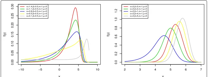
Figure4provides some plots of the density function (8) for selected parameter values. They reveal that this distribution is a good candidate to model left skewed and symmetric data sets.
Based on the LZBOLL-GHN density, we propose a linear location-scale regression model linking the response variable yi and the explanatory variable vector vi =
(vi1,. . .,vip)given by
yi=viβ+σzi, i=1,. . .,n, (11)
Fig. 4Plots of the LZBOLL-GHN density function for selected parameter values
location parameter vectorμ= (μ1,. . .,μn)is represented by a linear modelμ= Vβ, whereV=(v1,. . .,vn)is a known model matrix.
The LZBOLL-GHN model (11) provides new opportunities for modeling several types of data sets. This model contains two important regression models as its sub-models: (i) forβ = 1, the LZBOLL-GHN model reduces to log-OLL-GHN regression model intro-duced by Pescim et al. (2017); (ii) forα = β = 1, the LZBOLL-GHN model reduces to log-GHN regression model.
LetFandCbe the sets of individuals for whichyiis the log-lifetime or log-censoring, respectively. Assume that the observed lifetimes and censoring times are indepen-dent. The log-likelihood function for the vector of parameters = (α,β,σ,β) from model (11) is given byl() = 0
i∈F
li()+ 0 i∈C
l(ic)(), whereli() = log[f(yi)],
l(ic)()=log[S(yi)]. Thef(yi)andS(yi)are defined in(8) and (9), respectively. The total log-likelihood function foris given by
()=rlog
α
(β) σ√2π
−1
2 $
i∈F
expzi
√
2+
√
2 2
$
i∈F
zi
+(α−1)$ i∈F
log [ui−1]+(α−1) $
i∈F
log(2−ui)−2 $
i∈F
log[ui−1]α+(2−ui)α
+(β−1)$ i∈F
log 1
−log
(
2−ui)α
[ui−1]α+(2−ui)α 2
+$
i∈C
log 1
1− 1
(β)γ
β,−log
1− [ui−1] α
[ui−1]α+(2−ui)α 2
,
(12)
where ui = 2[ exp(zi
√
2/2)],zi = (yi−μi)/σ, andr is the number of uncensored observations (failures). The MLE'of the vector of unknown parameters can be evalu-ated by maximizing the log-likelihood (12). The R software is used to estimate unknown parameters of LZBOLL-GHN regression model
The likelihood ratio (LR) statistic can be used for comparing some sub-models of LZBOLL-GHN regression model. For example, the LR statistic can be used to dis-criminate between the LZBOLL-GHN and LGHN regression models since they are nested models, or equivalently to test H0 : α = β = 1. The LR statistic reduces to w = 2(αˆ,βˆ,σˆ,βˆ)−(1, 1,σ˜,β˜), whereαˆ,βˆ,σˆ,βˆare the unrestricted MLEs and
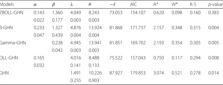
Table 2MLEs and their SEs of the fitted models and goodness-of-fit statistics for first data set
Models α β λ θ − AIC A* W* K-S p-value
ZBOLL-GHN 0.143 1.360 4.049 8.243 73.053 154.107 0.620 0.098 0.160 0.383
0.022 0.177 0.003 0.003
B-GHN 0.233 1.327 4.876 13.924 81.868 171.737 2.157 0.348 0.315 0.004 0.047 0.439 0.004 0.004
Gamma-GHN 0.238 4.945 13.941 81.851 169.702 2.193 0.354 0.305 0.005
0.042 0.003 0.003
OLL-GHN 0.165 4.016 8.488 75.522 157.043 0.750 0.117 0.294 0.008
0.032 0.141 0.133
GHN 1.491 10.226 87.927 179.853 3.074 0.521 0.278 0.014
0.255 0.903
n → ∞) distributed as χk2, where k is difference of two parameter vectors of nested models. For example, takek=2 for the above hypothesis test.
Residual analysis
Residual analysis has critical role to check the adequacy of the fitted model. In order to analyze departures from error assumption, two types of residuals are considered: martingale and modified deviance residuals.
Martingale residual
The martingale residuals is defined in counting process and takes values between+1 and−∞(see for details, Fleming and Harrington (1994)). The martingale residuals for LZBOLL-GHN model is,
rMi= ⎧ ⎨ ⎩
1+log
1−(β)1 γ
β,−log
1− [ui−1]α [ui−1]α+(2−ui)α
if i∈F,
log
1−(β)1 γ
β,−log
1− [ui−1]α [ui−1]α+(2−ui)α
if i∈C, (13)
whereui=2
exp
zi
√ 2/2
andzi=(yi−μi)/σ.
Modified deviance residual
The main drawback of martingale residual is that when the fitted model is correct, it is not symmetrically distributed about zero. To overcome this problem, modified deviance
(a) (b)
Table 3The LR test results for first data set
Hypotheses LR p-value
ZBOLL-GHN versus OLL-GHN H0:β=1 4.936 0.0262
ZBOLL-GHN versus Gamma-GHN H0:α=1 17.595 <0.0001
ZBOLL-GHN versus GHN H0:α=β=1 29.746 <0.0001
residual was proposed by Therneau et al. (1990). The modified deviance residual for LZBOLL-GHN model is,
rDi= ⎧ ⎪ ⎪ ⎪ ⎪ ⎨ ⎪ ⎪ ⎪ ⎪ ⎩
signˆrMi ⎧⎨
⎩−2 ⎡ ⎣
1+log1−(β)1 γβ,−log1− [ui−1]α
[ui−1]α+(2−ui)α
+log−log1−(β)1 γβ,−log1− [ui−1]α
[ui−1]α+(2−ui)α
⎤ ⎦ ⎫ ⎬ ⎭ 1 2
if i∈F,
signˆrMi −2
1+log1− 1
(β)γ
β,−log1− [ui−1]α
[ui−1]α+(2−ui)α
1
2
if i∈C,
(14)
whererˆMiis the martingale residual.
Applications
In this section, four real data sets are used to compare ZBOLL-GHN model with its sub-models and beta-GHN model introduced by Pescim et al. (2013). The first three data sets are used to demonstrate the univariate data fitting performance of ZBOLL-GHN distribu-tion. The fourth data set is used to investigate the usefulness of the proposed distribution in survival analysis. Theoptimfunction is used to estimate the unknown model parame-ters. The MLEs and corresponding standard errors, estimated−, Kolmogorov-Smirnov (K-S) statistic and corresponding p-value, Cramér-von Mises (W*), Anderson-Darling (A*) statistics and Akaike Information Criteria (AIC) are reported in Tables2,4and6. The lower the values of these criteria show the better fitted model on the data sets. The
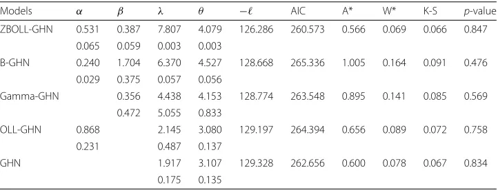
Table 4MLEs and their SEs of the fitted models and goodness-of-fit statistics for second data set
Models α β λ θ − AIC A* W* K-S p-value
ZBOLL-GHN 0.531 0.387 7.807 4.079 126.286 260.573 0.566 0.069 0.066 0.847
0.065 0.059 0.003 0.003
B-GHN 0.240 1.704 6.370 4.527 128.668 265.336 1.005 0.164 0.091 0.476 0.029 0.375 0.057 0.056
Gamma-GHN 0.356 4.438 4.153 128.774 263.548 0.895 0.141 0.085 0.569
0.472 5.055 0.833
OLL-GHN 0.868 2.145 3.080 129.197 264.394 0.656 0.089 0.072 0.758
0.231 0.487 0.137
GHN 1.917 3.107 129.328 262.656 0.600 0.078 0.067 0.834
0.175 0.135
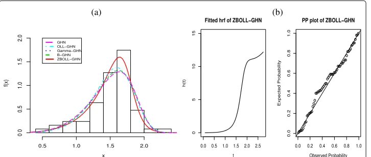
histograms with fitted pdfs are provided for visual comparison of the fitted distribution functions. Moreover, fitted hrfs and P-P plots of the best fitted models are displayed in Figs.5, 7and 9.
Lifetime of device data
The first data set is given by Sylwia (2007) on the lifetime of a certain device. Table2shows the estimated parameters and their standard errors,−, A*, W*, K-S and its corresponding p-value and AIC values. Based on the figures in Table2, it is clear that ZBOLL-GHN model provides the best fit for this data set. Figure5a displays the estimated pdfs of the fitted models. Figure5b displays the P-P plot of ZBOLL-GHN distribution and its fitted hrf. Figure5shows that ZBOLL-GHN distribution provides superior fit to the left-skewed data set.
Table3shows the LR statistics and the correspondingp-values for the first data set. From Table3, the computedp-values are smaller than 0.05, so the null hypotheses are rejected for all sub-models. We conclude that the ZBOLL-GHN model fits the first data better than its sub-models according to the LR test results.
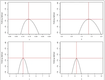
In addition, the profile log-likelihood functions of the ZBOLL-GHN distribution are plotted in Fig. 6. These plots reveal that the likelihood functions of the ZBOLL-GHN distribution have solutions that are maximizers.
(a) (b)
Table 5The LR test results for second data set
Hypotheses LR p-value
ZBOLL-GHN versus OLL-GHN H0:β=1 5.822 0.016
ZBOLL-GHN versus Gamma-GHN H0:α=1 4.976 0.026
ZBOLL-GHN versus GHN H0:α=β=1 6.084 0.047
Failure times of wind-shield data
The second data set represents the failure times for a particular wind-shield model includ-ing 85 observations that are classified as failed times of wind-shields (Murthy et al.2004). Table4shows the estimated parameters and their standard errors,−and AIC values. Based on the figures in Table4, ZBOLL-GHN distribution provides the best fit among others. Figure7a displays the histogram with fitted pdfs and Fig.7b displays the fitted hrf and P-P plot of ZBOLL-GHN distribution. These figures reveal that ZBOLL-GHN model provides superior fit to the second data set.
Table5shows the LR statistics and the correspondingp-values for the second data set. From Table5, the computedp-values are smaller than 0.05, so the null hypotheses are rejected for all sub-models. We conclude that the ZBOLL-GHN model fits the first data better than its sub-models according to the LR test results.
The profile log-likelihood functions of the ZBOLL-GHN distribution are plotted but not included here. These plots reveal that the likelihood functions of the ZBOLL-GHN distribution have solutions that are maximizers.
Strengths of glass fibres data
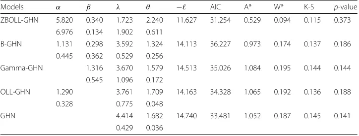
The third data set obtained from Smith and Naylor (1987) represents the strengths of 1.5 cm glass fibres, measured at the National Physical Laboratory, England. Unfortunately, the units of measurement are not given in the paper. This data set have been analyzed recently with the beta generalized exponential distribution, which was introduced and studied by Barreto-Souza et al. (2010). Table6shows the estimated parameters and their standard errors,−and AIC values. Based on the figures in Table6, ZBOLL-GHN dis-tribution provides the best fit among others. Figure8a displays the histogram with fitted pdfs and Fig.8b displays the fitted hrf and P-P plot of ZBOLL-GHN distribution. These figures reveal that ZBOLL-GHN model provides superior fit to the third data set.
Table7shows the LR statistics and the correspondingp-values for the third data set. From Table7, the computedp-values are smaller than 0.05, so the null hypotheses are
Table 6MLEs and their SEs of the fitted models and goodness-of-fit statistics for third data set
Models α β λ θ − AIC A* W* K-S p-value
ZBOLL-GHN 5.820 0.340 1.723 2.240 11.627 31.254 0.529 0.094 0.115 0.373 6.976 0.134 1.902 0.611
B-GHN 1.131 0.298 3.592 1.324 14.113 36.227 0.973 0.174 0.137 0.186 0.445 0.362 0.529 0.256
Gamma-GHN 1.316 3.670 1.579 14.513 35.026 1.084 0.195 0.144 0.144
0.545 1.096 0.172
OLL-GHN 1.290 3.761 1.709 14.163 34.328 1.065 0.192 0.136 0.188
0.328 0.775 0.048
GHN 4.414 1.682 14.740 33.481 1.052 0.187 0.145 0.141
Table 7The LR test results for third data set
Hypotheses LR p-value
ZBOLL-GHN versus OLL-GHN H0:β=1 5.0716 0.0243
ZBOLL-GHN versus Gamma-GHN H0:α=1 5.7716 0.0162
ZBOLL-GHN versus GHN H0:α=β=1 6.2264 0.0444
rejected for all sub-models. We conclude that the ZBOLL-GHN model fits the first data better than its sub-models according to the LR test results.
The profile log-likelihood functions of the ZBOLL-GHN distribution are plotted but not included here. These plots reveal that the likelihood functions of the ZBOLL-GHN distribution have solutions that are maximizers (Fig.8).
Voltage data
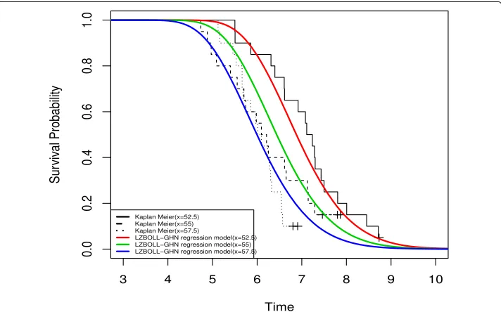
Lawless (2003) reported an experiment in which specimens of solid epoxy electrical-insulation were studied in an accelerated voltage life test. The sample size isn=60, the percentage of censored observations is 10% and there are three levels of voltage: 52.5, 55.0 and 57.5. The variables involved in the study are:xi- failure times for epoxy insula-tion specimens (in min);ci- censoring indicator (0 =censoring, 1 =lifetime observed);vi1
- voltage (kV).
The data set was used by Pescim et al. (2013) for illustrating the log-B-GHN (LBGHN) regression model. Pescim et al. (2013) compared the log-B-GHN (LBGHN) regression model with LOLLGHN and log-GHN (LGHN) models. In this section we compare the LZBOLL-GHN regression model with models reported in Pescim et al. (2013). The regression model fitted to the voltage data set is given by
yi=β0+β1xi1+σzi, (15)
where the random variableyi follows the LZBOLL-GHN distribution given in (8). The results are presented in Table8. The MLEs of the model parameters and their SEs and the values of the AIC and BIC statistics are listed in Table8.
Based on the figures in Table8, we conclude that the fitted LZBOLL-GHN regression model has the lowest AIC and BIC values. Figure9provides the plots of the empirical and
(a) (b)
Table 8MLEs of the parameters to the voltage data for LZBOLL-GHN, LBGHN, LGHN and log-Weibull regression models, the corresponding SEs in second line, p-values in third line and the AIC and BIC statistics
Model α β σ β0 β1 AIC BIC
LZBOLL-GHN 41.488 10.857 16.021 21.865 -0.177 166.264 176.735
49.967 11.306 18.828 11.003 0.063
0.047 0.005
LBGHN 102.140 1.564 5.306 10.632 -0.201 167.100 177.500
3.989 0.672 0.666 3.304 0.056
0.002 0.001
LGHN 0.778 23.637 -0.301 178.800 185.100
0.089 2.928 0.053
<0.001 <0.001
Log-Weibull 0.845 22.032 -0.275 173.400 179.700
0.090 3.046 0.055
<0.001 <0.001
estimated survival function for the LZBOLL-GHN regression model. We can conclude from these plots that LZBOLL-GHN regression model provides a good fit to the data.
Residual Analysis of LZBOLL-GHN model
Figure10displays the index plot of the modified deviance residuals and its Q-Q plot againstN(0, 1)quantiles. Based on the Figure10, we conclude that none of the observed values appears as a possible outlier. Thus, it is clear that the fitted model is appropriate for these data set (Fig.10).
(a) (b)
Fig. 10 aIndex plot of the modified deviance residual andbQ-Q plot for modified deviance residual
Summary
A new model called Zografos-Balarkishnan odd log-logistic generalized half-normal is introduced and studied. We assess the performance of the maximum likelihood estima-tors of the parameters of the new distribution with respect to the sample size n. The assessment is based on a graphical simulation study. The flexibility of the new model is illustrated by means of the three real data sets. The new model performs much better than beta generalized half-normal, generalized half-normal, odd log-logistic generalized half-normal and the generalized half-normal models. Additionally, a new log-location regression model based on the new distribution is introduced and studied. The martin-gale residual and the modified deviance residuals to detect outliers and evaluate the model assumptions are defined. We demonstrate that the new log-location regression model can be very useful in the analysis of real data and provide more realistic fits than other regres-sion models such as the log beta generalized half-normal, the log generalized half-normal and the log-Weibull regression models. The potentiality of the new regression model is illustrated by means of a real data.
Abbreviations
ALs: Average lengths; BGHN: Beta generalized half-normal; BGHNG: Beta generalized half-normal geometric; CPs: Coverage probabilities; GHN: Generalized half-normal; HN: Half-normal; KwGHN: Kumaraswamy generalized half-normal; LZBOLLGHN: Log-Zografos-Balarkishnan odd log-logistic generalized half-normal; MLEs: Maximum likelihood estimates; MSEs: Means square errors; OLLGHN: odd log-logistic generalized half-normal; ZBOLL-G: Zografos-Balarkishnan odd log-logistic-G; ZBOLLGHN: Zografos-Balarkishnan odd log-logistic generalized half-normal
Acknowledgments Not applicable.
Funding
GGH (co-author of the manuscript) is an Associate Editor of JSDA, 100% discount on Article Processing Charge (APC) for accepted article).
Availability of data and material
The used data sets are given in the manuscript.
Authors’ contributions
EA, HMY and GGH have contributed jointly to all of the sections of the paper. All authors read and approved the final manuscript.
Competing interests
The authors declare that they have no competing interests
Publisher’s Note
Author details
1Department of Statistics, Bartin University, Bartin 74100, Turkey.2Department of Statistics, Mathematics and Insurance, Benha University, Benha, Egypt.3Department of Mathematics, Statistics and Computer Science, Marquette University, Milwaukee, USA.
Received: 1 May 2018 Accepted: 4 November 2018
References
Aarts, R.M.: Lauricella functions (2000).www.mathworld.com/LauricellaFunctions.html. From MathWorld - A Wolfram Web Resource, created by Eric W. Weisstein
Barreto-Souza, W., Santos, A.H., Cordeiro, G.M.: The beta generalized exponential distribution. J. Stat. Comput. Simul.80, 159–172 (2010)
Cooray, K., Ananda, M.M.A.: A generalization of the half-normal distribution with applications to lifetime data. Commun. Stat. Theory Methods.37, 1323–1337 (2008)
Cordeiro, G.M., Alizadeh, M., Ortega, E.M., Serrano, L.H.V.: The Zografos-Balakrishnan odd log-logistic family of distributions: properties and applications. Hacettepe Res. J. Math. Stat.45, 1781–1803 (2016a)
Cordeiro, G.M., Alizadeh, M., Pescim, R.R., Ortega, E.M.M.: The odd log-logistic generalized half-normal lifetime distribution: properties and applications. Commun. Stat. Theory Methods.46, 4195–4214 (2016b)
Cordeiro, G.M., Pescim, R.R., Ortega, E.M.M.: The Kumaraswamy generalized half-normal distribution for skewed positive data. J. Data Sci.10, 195–224 (2012)
Cordeiro, G.M., Pescim, R.R., Ortega, E.M.M., Demétrio, C.G.B.: The beta generalized half-normal distribution: new properties. J. Probab. Stat.2013, 1–18 (2013)
Eugene, N., Lee, C., Famoye, F.: Beta-normal distribution and its applications. Commun. Stat. Theory Methods.31, 497–512 (2002)
Exton, H.: Handbook of hypergeometric integrals: theory, applications, tables, computer programs. Halsted Press, New York (1978)
Fleming, T.R., Harrington, D.P.: Counting process and survival analysis. John Wiley, New York (1994)
Hamedani, G.G.: On certain generalized gamma convolution distributions II (No. 484). Technical Report No. 484. Marquette University, MSCS (2013)
Lawless, J.F.: Statistical models and methods for lifetime data, Wiley Series in Probability and Statistics. Wiley, Hoboken, NJ, USA (2003). 2nd edition
Murthy, D.P., Xie, M., Jiang, R.: Weibull models (Vol. 505). Wiley (2004)
Pescim, R.R., Ortega, E.M., Cordeiro, G.M., Alizadeh, M.: A new log-location regression model: estimation, influence diagnostics and residual analysis. J. Appl. Stat.44, 233–252 (2017)
Pescim, R.R., Demetrio, C.G.B., Cordeiro, G.M., Ortega, E.M.M., Urbano, M.R.: The beta generalized half-normal distribution. Comput. Stat. Data Anal.54, 945–957 (2010b)
Pescim, R.R., Ortega, E.M.M., Cordeiro, G.M., Demetrio, C.G.B., Hamedani, G.G.: The log-beta generalized half-normal regression model. J. Stat. Theory Appl.12, 330–347 (2013)
Ramires, T.G., Ortega, E.M.M., Cordeiro, G.M., Hamedani, G.G.: The beta generalized half-normal geometric distribution. Stud. Sci. Math. Hung.50, 523–554 (2013)
Smith, R.L., Naylor, J.C.: A comparison of maximum likelihood and bayesian estimators for the three-parameter Weibull distribution. Appl. Stat.36, 358–369 (1987)
Sylwia, K.B.: Makeham’s generalised distribution. Comput. Methods Sci. Tech.13, 113–120 (2007)
Therneau, T.M., Grambsch, P.M., Fleming, T.R.: Martingale-based residuals for survival models. Biometrika.77, 147–160 (1990)