An Efficient Text Clustering Framework

An Efficient Text Clustering Framework

Francis M. Kwale

(Lecturer),

Department of Mathematics & Computer Science, University of Eldoret, P.O. Box 1125-30100,

ELDORET. KENYA.

ABSTRACT

The amount of data for analysis is increasing at a dramatic rate, for example web data. And so, it’s important to improve techniques of searching relevant information from the huge data so as to increase efficiency. One such technique is text clustering, whereby we group (or cluster) text documents into various groups (or clusters), such as clustering web search engine results into meaningful groups. Data mining is a computer science area that can be defined as extraction of useful information from large structured data. Text mining on the other hand is an extension of data mining dealing only with (unstructured) text data. Text clustering is thus a text mining technique. In this paper, we give an insight of text clustering including the text mining related areas, techniques, and application areas. We also propose a framework for doing text clustering based on the K Means algorithm. The paper thus gives guidance to researchers of text mining concerning the state of art of text clustering.

Keywords: clusters, data mining, structured, text clustering, text mining, unstructured.

1. INTRODUCTION

1.1 Data Mining (DM) and Text Mining

(TM)

Data mining can be defined as extraction of useful information from large (structured) data sets. By observing large data sets over a period of time, we can deduce previously-unknown and useful information concerning patterns, models, trends, and rules in the area of application. For example, from a sales database of a retail company observed over a longer period of time, we can deduce that item x goes with item y, a particular item is mostly purchased during a particular time of the year, etc. A lot of research has already been done on it. However, data mining can be applied only on structured data (e.g. databases with well defined fields, making information searching easier). It cannot be applied on unstructured data (e.g. text documents, web documents) that is often fuzzy and ambiguous and thus hard to draw patterns, trends, directions, rules, etc.

Since the most natural form of storing data is in form of text documents (i.e. unstructured data), we must apply text mining to extract useful information. Unfortunately, for many applications, electronic information is only available in the form of free natural-language documents rather than structured databases [26], p. 1. Text mining thus, is believed to have a commercial potential higher than that of data mining.

Text mining refers to the process of extracting useful and non-trivial patterns or knowledge from unstructured text.

Being an extension of data mining, it’s also known as text data mining or knowledge discovery from textual databases. TM can be applied to detect patterns, models, trends, or rules from unstructured data. It is more complex task than data mining since it deals with text data that are inherently unstructured, ambiguous and fuzzy. Text mining is an interdisciplinary area borrowing from other areas including information retrieval, machine learning, statistics, computational linguistics and especially data mining.

1.2 Text Mining Techniques

Two typical data mining (and also TM) techniques are classification and clustering.

Classification technique assigns pre-defined classes to data sets. It thus works in a supervised manner. For example, we can label each message of an opinion poll in one of the classes “Accept”, “Reject”, or “No answer”. The classification starts with training a set of data that are already labeled with a particular class (e.g. “Accept”). It then determines a classification model which is able to assign the correct class to a new data of the area of application.

Clustering on the other hand is used to group data sets with similar content. Text document clustering is a text mining technique which divides the given set of text documents into significant clusters [33], p. 1. Clustering technique doesn’t use predefined topics unlike classification, but instead clusters documents based on similarity to each other. It thus works in an unsupervised manner. For example, web search engine produces a group of document talking about different previously unknown topics. We can consequently group (or cluster) the documents into the different unknown topics, and so this can’t be supervised.

1.3 Applications of Text Clustering

Some of the many possible applications of text clustering include; improving precision and recall in information retrieval [37], p. 4, organizing of web engine search results into meaningful groups, web filtering (removing unwanted web materials), in marketing (e.g. grouping Customer Relationship Management (CRM) correspondence), in opinion poll mining (e.g. grouping opinions into the possible groups), bioinformatics (e.g. identifying and classifying molecular biology terms corresponding to instances of concepts under study by biologists), land use: identification of areas of similar land use in an earth observation database [35], p. 18, image processing, and pattern recognition.

1.4 Text Complexity

modes (e.g. it has different natural languages, and different formats); often contains ambiguity (e.g. polysemy - a word having different meanings e.g. “bank”: river bank or financial institution, synonyms - many words with same or similar meaning depending on the area of application e.g. “singer” and “vocalist”); is unstructured i.e. whereas structured data has a particular organization, e.g. a set of numeric values (with a particular data type and size), a database (with a particular organization/structure i.e. known fields with fixed data types and sizes), text documents are freely occurring plain text messages with no organization/structure, and so are said to be unstructured; and text suffers from high dimensionality (text documents may contain tens of thousands of words, yet only a very small percentage is used in a typical document).

2. THE TEXT CLUSTERING

FRAMEWORK

2.1 The Text Clustering Approach

Applying data mining techniques is simple and straightforward since the data is structured. But when dealing with unstructured text documents, we can’t apply the traditional data mining techniques straight. But if we could get a way of converting the unstructured text documents into a structured form, we could then simply apply the traditional data mining techniques (e.g. clustering) on the resulting structure. This is the usual approach in text clustering.

Thus, the text clustering approach is to remove the text complexities explained in section 1.4, and then apply the traditional and simpler/known data clustering technique on the resulting structured database, i.e.

1. Preprocessing: Here, we remove high-dimension-causing words from the text document i.e. unnecessary words that cause unimportant high dimensions (e.g. introductory words like headings, punctuation marks like commas, frequent words like “the”, “of”, “and”, etc), as well as complexities (e.g. resolving words with multiple meanings). This makes the text simpler/easier to structure. For example, removal of too frequent and unimportant words like “and” makes the resulting text simpler and easier to structure.

2. Transformation: We convert the resulting ‘more direct and easy to structure’ text into a structured form and store this into a structure, e.g. a matrix.

3. Clustering: We apply the traditional data mining clustering on the resulting structure.

2.2 The Proposed Framework

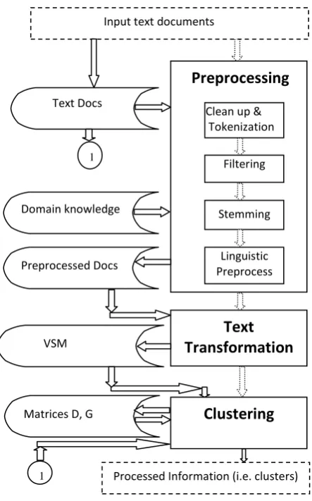
We thus, propose the text clustering process as depicted by the following figure.

Fig 1: A text clustering technical architecture

The domain knowledgebase contains existing already-known rules on text (e.g. usage of words depending on the language e.g. English). The text documents store contains the text documents being clustered. The preprocessed documents store contains the preprocessed documents. The VSM stores the documents data inform of vector space model (VSM) i.e. the term-document matrix. The matrices D ands G are distance and group matrices used during clustering phase. The phases are explained below.

2.2.1 Preprocessing

The aim of preprocessing is to remove complexities from the text documents. There sequence of techniques involved here are: Text clean up, tokenization, filtering, stemming, and linguistic preprocessing.

1. Text cleanup: This initial technique removes document parts that are not relevant to interpreting the document’s content, e.g. removes adverts from web pages, normalizes text converted from binary formats, deals with tables, figures and formulas, etc. For example in an opinion poll, a text message starting as “I wish to give my opinion. Mr XYZ has done an excellent job in …” need not have the portion “I wish to give my opinion” included.

2. Tokenization: This is done so as to obtain a stream of only important words by;

 Removing punctuation marks e.g. commas (,), semi colons (;), hyphens (-), etc, since they are considered inconsequential.

Input text documents

Input text documents

Processed Information (i.e. clusters)

Preprocessing

Clean up & Tokenization

Filtering Stemming

Linguistic Preprocess ing

Text

Transformation

Clustering

Do Domain knowledge T ext Text Docs

T ext Preprocessed Docs

VSM

T Matrices D, G

111

1

11

1

111

 Replacing tab spaces and other non-text characters with single spaces, since tabs have no meaning.

For example, the message “We should elect john, Paul” is converted into “We should elect John Paul”. Similarly, “data-base” is converted into “data “data-base”. This forms the dictionary of a document collection.

3. Filtering: Filtering technique aims at reducing the size of the dictionary and thus, the size of the description of documents in question. Filtering removes unimportant or less important words (also known as stop words) including;

 Prepositions and conjunctions, e.g. “the”.

 Words occurring extremely frequently as well as words occurring very rarely.

These are also believed to have very little or no statistical relevance. For example, the words “the”, “of”, “a”, “to”, “I”, etc occur very frequently in documents and also have very little or no relevance to distinguishing, relating or classifying of different messages. Also, words that occur very rarely are not likely to have statistical relevance.

4. Stemming: Stemming technique tries to build the basic forms of words (or reduce words into their form), and thus, simplifies the text messages. The technique strips plurals from nouns, “ing” from verbs, “s” from words, as well as other affixes. For example, “electing James” becomes “elect James”, “Peter’s” becomes “Peter”, etc. This produces a stem of words. A stem is a group of words with same/similar meaning, e.g.

 “user”, “use”, “using” are similar and may be stemmed to “use”.

 “agreed”, “agreeing”, “agreement” have similar meaning and may be stemmed to “agree”.

5. Linguistic Preprocessing: These are additional preprocessing methods used to enhance the available information. They include;

 Part of speech tagging that determines the part of a speech, e.g. noun, verb, adjective, etc for each term. It marks up the words in a text with their corresponding parts of speech.

 Text chunking that groups adjacent words in a text.

 Word Sense Disambiguation (WSD) that resolves ambiguities in words, including multiple meanings words, e.g. “pen”. The technique determines in which sense a word having a number of distinct senses is used in a given sentence.

Example

We use the following simple example of three documents to illustrate the above steps (except linguistic preprocessing). Remember the problem is clustering the three documents.

D1: My professional advice to all is this: Fruits are very healthy.

D2: Doctor’s Recommendations

Please give your infant fruit, since this is good for the infant’s health.

D3: Exercising is healthier.

Text clean up: Here we remove the heading “My

professional advice to all is this:” from D1 and “Doctor’s

Recommendations” from D2, since they are not important in the clustering.

Tokenization: We remove the quote (’) and the comma (,) from D2, and full stops from D1, D2, D3.

Filtering: We remove unimportant words that don’t form any

basis in clustering. These are “are”, “very” from D1, “Please”, “give”, “your”, “since”, “this”, “is”, “good”, “for”, “the” from D2, and “is” from D3.

Stemming: We can stem

 “Fruits” and “fruit” into “fruit”,

 “infant” and “infants” into “infant”,

 “Exercising” into “exercise”, and

 “healthy”, “heath”, and “healthier” into “heath”

The resulting preprocessed documents will be

D1: fruit health

D2: infant fruit infant health

D3: exercise health

2.2.2 Text Transformation

After preprocessing, the resulting text is represented using an appropriate structured model, typically the vector space model.

1 The

Vector

The simplest implementation of the VSM is the Boolean model, whereby a document is regarded simply as a “bag of

words” (i.e. a set of words). In mathematics, a bag, also called a multiset, is a set with duplicates allowed [30], p. 7. Here, a collection of n documents containing m terms (or words) is represented using a matrix of m rows and n columns. So the rows represent the terms and the columns represent the documents. In other words, the rows are term vectors while the columns are document vectors. The ijth entry in the matrix is either a 1 (if the ith term is present in the jth document), or a 0 (if not). Thus, this ‘term-document’ matrix is said to be a “bag of words” since it contains repetition of values 1 and 0.

In space-based view, a document will be a data point in a high dimensional space, whereby each term is an axis of the space. Thus, the dimension of the space represents the number of terms in consideration, e.g. three terms will be represented by the xyz space, and two terms by the xy plane. And in the

xyz space, a document containing the first and the third terms will be represented by the point (1, 0, 1).

Example

We use the example of three preprocessed documents in section 2.2.1 above which are

D1: fruit health

D2: infant fruit infant health

D3: exercise health

Here, the first row is the vector (1, 1, 0) representing the first term (fruit), showing that the term occurs in the first and the second document, but not in the third. Similarly, the vector (1, 1, 0, 0) represents the first document (that contains the first and the second terms, but not the third and the fourth terms). And entry A42 is 0, showing that the fourth term (exercise) is

not present in the second document.

The advantages of the Boolean model are that the implementation is simple and straight forward. Also, this model immediately matches the computer-based Boolean algebra making searching to be simple and fast. Its limitation is that it is limited in that the relevance of a term in a document is a binary decision (i.e. either term occurs or not). It doesn’t cater for level of importance of the term in a document, e.g. more frequent terms in a document may be more important.

2 Modification of the VSM to Use Frequencies

The limitation of Boolean model of that the relevance of a term is a binary decision made it necessary to modify the VSM such that we use word frequencies. Here, the ijth entry in the term-document matrix represents the frequency of the ith

term in the jth document. This provides more information about terms.

Example 1

Using the example in section 1 above, the term-document matrix using frequencies is

The difference is that the third term (infant) occurs twice in the second document.

Example 2

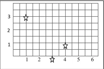
Assume we have documents D1, D2 and D3 containing two terms T1 and T2. Assume also that T1 occurs four times in D1, once in D2, and thrice in D3, while T2 occurs once in D1, thrice in D2, and zero times in D3. The term-document matrix therefore, is

And our space-based view is

Fig 2: Space-based view of three text documents, two terms

This is because as explained above, in space-based view, a document will be a data point in a high dimensional space, whereby each term is an axis of the space. Thus, our view has two dimensions (for the two terms) i.e. the xy plane (we let x

axis represent the first term, and y axis represent the second term). So the three documents will be the points (4, 1), (1, 3), and (3, 0) on the xy plane as illustrated below.

This approach has advantage over VSM in that it addresses the level of importance of a term in a document. However it does not take into account weighting information of terms. For example, a term could be very frequent in a document collection but may not be as appropriate as another infrequent term in terms of distinguishing a document from the rest. Thus, we have a third approach that takes into account weighting information of terms.

3 Modification of the VSM to Use Weights

The term weighting techniques assume that;

 Content-carrying words that are more frequent in a document are usually more meaningful than those that occur less frequently.

 Words that are more frequent in a document collection are usually less meaningful than those that occur less frequently.

In this case, three factors are used in term weighting:

 Local Term Factor (LTF): It weights a word based on its frequency (i.e. tf) within a document, i.e. the more frequent it is the higher the LTF. Popular formulae used here are

LTF=tf, LTF=log(1+tf).

 Global Term Factor (GTF): It weights a word based on its frequency within the document corpus. A popular formula used here is GTF=log(N/n), where N is the total number of documents in the corpus and n denotes the number of the documents in which the specific term occurs.

 Normalization Factor (NF): This takes care of the effect of the document’s length. It reduces the effect of a long document being unnecessarily more important than others concerning a term occurring many times in it, i.e. caters for documents with different lengths. Normalized vectors are also easier to deal with (since the range of their values is small, e.g. orthonomal vectors below), yet they retain the differences in documents.

One normalization formula is converting a document’s vector into an orthonormal vector i.e. by dividing it by its length. Thus, a document vector X=(x1, x2, …, xm) is normalized by dividing each of its elements by the vector’s length, i.e.

1 1 0 1 1 1 0 1 0 0 0 1

A =

4 1 3 1 3 0

A =

1 1 0 1 1 1 0 2 0 0 0 1

A =

1 2 3 4 5 6

xi ( xi÷√ ∑(xi )2 )

This results to unitary vectors, whereby the term values are between 0 and 1.

A term can be represented using all (or some of) the three factors, e.g. using LTF+GTF+NF

Example

Consider the term-document matrix in section 2 above, i.e.

(i) Local term factor (LTF)

Terms occurring 0 times in the matrix have LTF=log(1+0)=0, those occurring once have LTF=log(1+1)=0.301, and that occurring twice has LTF=log(1+2)=0.477. Thus, the LTF matrix is

This obviously implies that the term occurring many times (e.g. twice in this case) in a document is more important, and so has a high LTF

(ii) Global term factor (GTF)

The first term occurs in two out of the three documents, and thus, has a GTF of log(3/2)=0.176. The second term occurs in three documents, and thus, has a GTF of log(3/3)=0. The third term occurs in one document, and thus has a GTF of log(3/1)=0.477. Finally, the fourth term occurs in one document, and thus has a GTF of log(3/1)=0.477. Thus, the GTF matrix is

Thus, the term occurring in one document is more important globally than that occurring in two or three documents. The one occurring in all the three documents has GTF=0, meaning that it’s not important in distinguishing (and so clustering) the documents. I.e., all the three documents contain the word “health” meaning all are about health matters, and so we can’t do clustering based on that word. So, less frequent terms are important in distinguishing documents.

(iii) Normalization factor (NF)

The length of vector (1, 1, 0, 0) is (12+12+02+02) 0.5=1.414, the length of vector (1, 1, 2, 0) is (12+12+22+02) 0.5=2.449, while the length of vector (0, 1, 0, 1) is (02+12+02+12) 0.5=1.414

Thus, the three normalized vectors (after dividing each vector by its length) are (0.707, 0.707, 0, 0), (0.408, 0.408, 0.817, 0), and (0, 0.707, 0, 0.707). And the new term-document matrix (using only NF) becomes

It is clear that this matrix’s values are easier to deal with (since their range is 0 to 1), yet the differences of documents based on the words is maintained. For example in second document, first and second term have a weight of 0.408, while third term has 0.817, which clearly represents the same relationships as in the un-weighted matrices discussed above. This would also reduce the unnecessarily big importance of a frequent word in a very long document (since the most important thing is clustering documents into groups based on whether a word occurs in a document or not).

(iv) The weighting factor

Our weighting factor now becomes

Thus, the three documents will be represented using the immediate above matrix.

2.2.3 Clustering

After transformation of the unstructured documents into a structured form (e.g. into a VSM), clustering is then performed using appropriate algorithms. We will explain and illustrate the clustering using the K Means algorithm because it’s simple and easy to implement, and also efficient in execution. Various clustering algorithms exist, and can be classified on two bases, i.e.

 The organization of the resulting clusters, i.e. whether

hierarchical or flat.

 The approach used, i.e. the method used to determine which cluster a particular document belongs to. An example is the distance measurements approach whereby the algorithm works by measuring distances between document points in the VSM.

1. Hierarchical versus Flat (or Partitioning) Clustering Algorithms

Hierarchical-type algorithms produce tree-like clusters, with the root of the tree (the bottom most clusters) being the lowest level cluster, while the leaves of the tree (at the top) being the highest level clusters. Hierarchical techniques produce a nested sequence of partitions, with a single, all inclusive cluster at the top and singleton clusters of individual points at the bottom [36], p. 3. The produced tree structure is also known as a dendogram.

According to [36], p. 4, flat-type clusters produce one-level (i.e. un-hierarchical) partitions of documents. They usually receive the expected number of clusters as a parameter. The most widely used flat algorithm is the K-means algorithm.

2. Distance Measurement

We have seen from above that in VSM’s space-based view, a document will be a data point in a high dimensional space, whereby each term is an axis of the space. Consequently in a distance-based approach, the distance between two points in the space represents the measure of (dis)similarity between

1 1 0 1 1 1 0 2 0 0 0 1

0.707 0.408 0 0.707 0.408 0.707

0.301 0.301 0 0.301 0.301 0.301 0 0.477 0 0 0 0.301

0.176 0.176 0.176 0 0 0 0.477 0.477 0.477 0.477 0.477 0.477

0.707 0.408 0 0.707 0.408 0.707 0 0.817 0 0 0 0.707

0.176 0.176 0.176 0 0 0 0.477 0.477 0.477 0.477 0.477 0.477 0.301 0.301 0

0.301 0.301 0.301 0 0.477 0

0 0 0.301

+

+

=

1.184 0.885 0.176 1.008 0.709 1.008 0.477 1.771 0.477 0.477 0.477 1.485

the two documents. This means the length of the straight line between the two points, i.e. the Euclidean measure.

3. The K Means Algorithm

The K-Means algorithm is among the few most popular clustering algorithms, and has several variations. It was developed by J. MacQueen in 1967. It’s a partitioning, distance-based algorithm whose objective is to minimize the average squared Euclidean distance of documents from their cluster centers where a cluster center is defined as the mean or centroid of the documents in a cluster. According to [29], p. 2, the K Means algorithm assigns each point to a cluster whose center (also called centroid) is nearest. The centroid of a cluster is the average of all the points in the cluster based on the Euclidian distance measure.

The steps of the algorithm are.

1. Choose the number of clusters, k.

2. Randomly generate k clusters and determine the cluster centers (centroids).

3. Repeat the following until no object moves (i.e. no object changes clusters)

(i) Determine the distance of each object to all centroids.

(ii) Assign each point to the nearest centroid.

(iii) Re-compute the new cluster centers.

Thus, in each loop of step 3 above, the algorithm aims at minimizing the following function for k clusters and n data points.

j=k i=n

J=∑ ∑ ||x

-c

||

j=1 i=1

where ||xi-cj|| is a choosen distance measure between data point xi from cluster cj.

Example

Remember from section 2.2.2, we transformed the three text documents into the following structured representation (a term-document matrix) i.e. using the VSM

We could apply the above steps of K Means on this matrix, but we won’t be able to illustrate the clustering graphically since there are four terms in the matrix and hence four dimensions in the space-based view.

Therefore for simplicity, let’s use another example that contains only two terms, so that we illustrate the clustering graphically on the xy plane.

Assume four documents containing two terms, whereby the first term occurs with frequencies 1, 0, 4, and 6 respectively in the documents, while the second term occurs with frequencies 2, 2, 1, 0 respectively. Thus, the four document vectors are (1, 2), (0, 2), (4, 1), and (6, 0), i.e. with term-document matrix

We choose k=2, and the first two points (i.e. (1, 2), (0, 2)) as the initial first and second centroids.

First loop

We compute the distance matrix D (containing distance of each point from each centroid) to be

The first row of D shows the distance of each point from the first centroid, and the second row shows the distance of each point from the second centroid.

Here, the point (1, 2) has distance ((1-1)2+(2-2)2)1/2=0) from centroid (1, 2), and distance ((1-0)2+(2-2)2)1/2=1) from centroid (0, 2).

The point (0, 2) has distance ((0-1)2+(2-2)2)1/2=1) from centroid (1, 2), and distance ((0-0)2+(2-2)2)1/2=0) from centroid (0, 2).

The point (4, 1) has distance ((4-1)2_+(1-2)2₎1/2_{=3.16) from} centroid (1, 2), and distance ((4-0)2+(1-2)2)1/2=4.12) from centroid (0, 2).

The point (6, 0) has distance ((6-1)2+(0-2)2)1/2=5.39) from centroid (1, 2), and distance ((6-0)2+(0-2)2)1/2=6.33) from centroid (0, 2).

We then form the clusters by assigning each point to its nearest centroid. We form the group matrix G by assigning each point value 1 (if it should belong to that cluster), and value 0 if not. Note that first row represents the first cluster, and second row the second cluster. E.g., the third point (4, 1) has distance 3.16 from the first centroid, and distance 4.12 from the second centroid, meaning it’s nearer to the first centroid. So we set the third column of G below to (1, 0). Thus,

This shows that the first, third and fourth points belong to the first cluster, and the second point to the second cluster.

We then recompute the centroid of each cluster as the average of the points in that cluster. Thus, the new first centroid is ((1+4+6)/3, (2+1+0)/3) which is (3.67, 1), while the second centroid is (0, 2).

Second loop

We then start the second loop of the algorithm and compute D

to be

Here, the point (1, 2) has distance ((1-3.67)2+(2-1)2)1/2=2.85) from centroid (3.67, 1), and distance ((1-0)2+(2-2)2)1/2=1) from centroid (0, 2).

The point (0, 2) has distance ((0-3.67)2+(2-1)2)1/2=3.80) from centroid (3.67, 1), and distance ((0-0)2+(2-2)2)1/2=0) from centroid (0, 2).

1 1 0

1 1 1

0 2 0

0 0 1

A =

2.85 3.80 0.33 2.54 1 0 4.12 6.33

D

=

1 0 1 1 0 1 0 0

G

=

1 0 4 6

2 2 1 0

0 1 3.16 5.39 1 0 4.12 6.33

A =

The point (4, 1) has distance ((4-3.67)2+(1-1)2)1/2=0.33) from centroid (3.67, 1), and distance ((4-0)2+(1-2)2)1/2=4.12) from centroid (0, 2).

The point (6, 0) has distance ((6-3.67)2+(0-1)2)1/2=2.54) from centroid (3.67, 1), and distance ((6-0)2+(0-2)2)1/2=6.33) from centroid (0, 2).

Thus, the first point changes into the second centroid/cluster since it’s now distance 2.85 from the first centroid (3.67, 1) compared to distance 1 from the second centroid (0, 2). We therefore compute the new group matrix to be

We then recompute the centroid of each cluster as the average of the points in that cluster. Thus, first centroid is ((4+6)/2, (1+0)/2) which is (5, 0.5), while the second centroid is ((1+0)/2, (2+2)/2) which is (0.5, 2).

Third loop

We start the third loop of the algorithm and compute D to be

Here, the point (1, 2) has distance ((1-5)2+(2-0.5)2)1/2=4.27) from centroid (5, 0.5), and distance ((1-0.5)2+(2-2)2)1/2=0.5) from centroid (0.5, 2).

The point (0, 2) has distance ((0-5)2+(2-0.5)2)1/2=5.22) from centroid (5, 0.5), and distance ((0-0.5)2+(2-2)2)1/2=0.5) from centroid (0.5, 2).

The point (4, 1) has distance ((4-5)2+(1-0.5)2)1/2=1.11) from centroid (5, 0.5), and distance ((4-0.5)2+(1-2)2)1/2=3.64) from centroid (0.5, 2).

The point (6, 0) has distance ((6-5)2+(0-0.5)2)1/2=1.11) from centroid (5, 0.5), and distance ((6-0.5)2_+(0-2)2₎1/2_{=5.85) from} centroid (0.5, 2).

Thus,

And so there is no change of the clusters, and so we stop.

Illustration of the clustering

Remember our original matrix was

We can illustrate the immediate above clustering example using the space-based view as follows. Since there are two terms, we have a two dimensional space whereby x axis represents the first term while y axis represents the second term. Each document is a point on the xy space.

Note that;

 Document points are shown using

 Centroids are shown using or (if they are also data points)

 Points inside a cluster are enclosed using

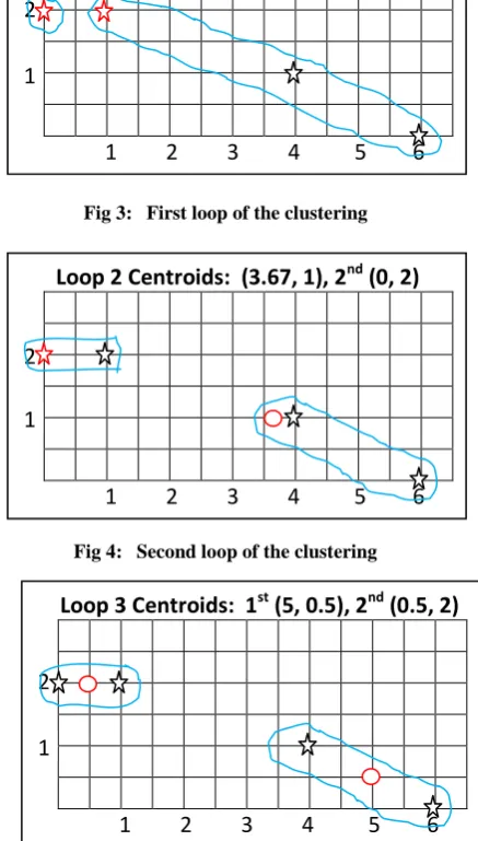
Fig 3: First loop of the clustering

Fig 4: Second loop of the clustering

Fig 5: Third loop of the clustering

Conclusion

The first two points i.e. (1, 2), (0, 2) are in the second cluster while the last two points i.e. (4, 1), and (6, 0) are in the first cluster.

3. CONCLUSIONS

The typical applications of text clustering (e.g. web searching) require fast response times to make clustering meaningful to the user. However, clustering of text documents is usually a difficult task involving complex computations. In fact, most text clustering algorithms currently used suffer from the limitation of inefficiency due to the complex logic.

Clearly, the above preprocessing and the VSM are direct and straightforward to implement. Also, it’s evident that the clustering steps using K Means in the above example (in section 2.2.3) are simple to follow and implement since they

0 0 1 1 1 1 0 0

G

=

0 0 1 1 1 1 0 0

G

=

4.27 5.22 1.11 1.11 0.5 0.5 3.64 5.85

6.33

D

=

1 0 4 6

2 2 1 0

A =

Loop 1 Centroids: 1

(1, 2), 2

(0, 2)

1 2 3 4 5 6

1

2

Loop 2 Centroids: (3.67, 1), 2

(0, 2)

1 2 3 4 5 6

1

2

Loop 3 Centroids: 1

(5, 0.5), 2

(0.5, 2)

1 2 3 4 5 6

1

use elementary data storage using matrices and simple matrices calculations. Also, the steps are clearly efficient to implement (only three simple-logic loops fully clustered the data, each loop involving a few expressions and assignment statements). In fact, K Means has a linear complexity.

Thus, the above described framework is recommended to be used in achieving a simple and efficient clustering system.

However, more needs to be done specifically to reduce the dimensions of the VSM. For example, assuming a typical application yields 1,000 documents to be clustered resulting to 500,000 terms, this means a term-document matrix of 500,000 rows and 1,000 columns which takes a lot of memory space. This thus, reduces the efficiency of the framework. Thus, we intent to explore ways of combining the K Means approach with another similarly simple and efficient dimension reduction approach.

4. REFERENCES

[1] Alelyani, S., Tang, J., and Liu, H. Feature selection for clustering: A review. Online notes, unpublished.

[2] Andrews, N., and Fox, E. Recent developments in document clustering. Technical Report, Department of Computer Science, Virginia Tech, viewed 31 January 2013.

<http://eprints.cs.vt.edu/archive/00001000/01/docclust.p df> unpublished.

[3] Bharathi, G., and Venkatesan, D. 2012. Study of ontology or thesaurus based document clustering and information retrieval. Journal of Theoretical and Applied Information Technology. Vol. 40, no. 1.

[4] Boomija, M., 2008. Comparison of partition based clustering algorithms. Journal of Computer Applications, Vol. 1, no. 4.

[5] Chen, C., Tseng, F., and Liang, T. 2010. Mining fuzzy frequent item sets for hierarchical document clustering. Information Processing and Management. Vol. 46, no. 2, pp. 193–211.

[6] Chifu, E. 2010. Self organizing maps in web mining and semantic web, PhD Thesis, Technical University of Cluj-Napoca.

[7] Chitsaz, E., Taheri, M., Katebi S., and Jahromi M. 2009. An improved fuzzy feature clustering and selection based on chi-squared test. Proceedings of the International MultiConference of Engineers and Computer Scientists 2009. Vol. I, IMECS 2009, March 18 - 20, 2009, Hong

Kong, viewed 14 July 2013,

<http://www.iaeng.org/publication/IMECS2009/IMECS2 009_pp35-40.pdf>

[8] Chu, S., Roddick, J., Pan, J. Improved search strategies and extensions to K-medoids-based algorithms. Technical Report KDM-02-005, School of Informatics and Engineering Flinders University of South Australia,

viewed 24 June 2013,

<http://kdm.first.flinders.edu.au/KDMTR/KDM02005.pd f> unpublished.

[9] Fung, B. 1999. Hierarchical document clustering using frequent item sets. MSc Thesis, Simon Fraser University, 1999.

[10] Geraci, F. 2008. Fast clustering for web information retrieval. PhD Thesis, Universit’ A Degli Studi Di Siena.

[11] Gruber, T. 1995. Toward principles for the design of ontologies used for knowledge sharing. International Journal Human-Computer Studies. Vol. 43, nos. 5-6, pp. 907-928.

[12] Guduru, N. 2006. Text mining with support vector machines and non-negative matrix factorization algorithms. MSc Thesis, University of Rhode Island.

[13] Hao, Z. 2012. A new text clustering method based on KGA. Journal of Software. Vol. 7, no. 5, pp. 1-5.

[14] Hotho, A., Maedche, A., and Staab, S. 2001. Ontology-based text document clustering. Proceedings of the Workshop “Text Learning: Beyond Supervision” at IJCAI 2001 Seattle WA USA, August 6, 2001. Viewed 05 February 2013, <http://www.aifb.uni-karlsruhe.de/WBS> unpublished.

[15] Jayabharathy, J., Kanmani, S., and Parveen, A. 2011. A s u r v e y o f d o c u m e n t c l u s t e r i n g a l g o r i t h m s w i t h t o p i c d i s c o v e r y . Journal of Computing. Vol. 3, no. 2, pp. 1-3.

[16] Khan, L. 2000. Ontology-based information selection. PhD Thesis, University of Southern California.

[17] Krishna, B., Satheesh, P., and Kumar, S. 2012. Comparative study of K-means and Bisecting K-means techniques in Wordnet-based document clustering. International Journal of Engineering and Advanced Technology. Vol 1, no 6, pp 1-4.

[18] Langville, A. and Meyer, C. Text mining using the nonnegative matrix factorization. SIAM-SEAS– Charleston, 2005, unpublished.

[19] Lasek, P. 2011. Efficient density-based clustering. PhD Thesis, Warsaw University of Technology.

[20] Lee, S., Song, J., and Kim, Y. An empirical comparison of four text mining methods. Journal of Computer Information Systems, 2010, unpublished.

[21] Liu, T., Liu, S., Chen, Z., and Ma, Z. 2003. An evaluation on feature selection for text clustering. Paper presented at proceedings of the Twentieth International Conference on Machine Learning (ICML-2003), Washington DC.

[22] Li, Y., 2007. High performance text document clustering. PhD Thesis, Wright State University.

[23] Li, Y., Congnan, L., and Soon, M. 2008. Text clustering with feature selection by using statistical data. IEEE Transactions on Knowledge and Data Engineering, vol. XX, no. YY.

[24] Magatti, D. 2010. Graphical models for text mining: knowledge extraction and performance estimation. PhD Thesis, UNIVERSITÀ DEGLI STUDI DI MILANO – BICOCCA.

[25] Moldovan, D., and Novischi, A. 2004. Word sense disambiguation of WordNet glosses. Elsevier Ltd, 2004,

viewed 16 June, 2013,

<www.hlt.utdallas.edu/~moldovan/newpapers/j04dman.p df > unpublished.

January 2013, <http://www.cs.utexas.edu/users/ml/papers/discotex-melm-03.pdf>

[27] Ng, R., and Han, J. 2002. CLARANS: A method for clustering objects for spatial data mining. IEEE Transactions on Knowledge and Data Engineering. Vol. 14, no. 5.

[28] Ning, W. 2005. Text mining and organization in large corpus. MSc Thesis, Technical University of Denmark (DTU).

[29] Punitha, S., and Punithavalli, M. 2012. A comparative study to find a suitable method for text document clustering. IJCSNS International Journal of Computer Science and Network Security. Vol. 12, no. 10.

[30] Rehurek, R. 2011. Scalability of semantic analysis in natural language processing. PhD Thesis, Masaryk University.

[31] Rai, P. 2010. A survey of clustering techniques. International Journal of Computer Applications. Vol. 7, no 12.

[32] Rosell, M., “Clustering exploration: Swedish text representation and clustering results unraveled”, PhD Thesis, Stockholm, Sweden, 2009.

[33] Sharma, S., and Gupta, V. 2012. Recent development in text clustering techniques. International Journal of Computer Applications (0975 – 8887). Vol. 37, no. 6, pp. 1-5.

[34] Sree K., and Murthy J. 2012. Clustering based on cosine similarity measure. International Journal of Engineering Science & Advanced Technology. Vol 2, no 3, pp 1-2.

[35] Stefanowski, J. Data mining clustering. Online lecture

notes”, 2009, viewed 10 June 2013,

<http://www.cs.put.poznan.pl/jstefanowski/sed/DM-7clusteringnew.pdf.> unpublished.

[36] Steinbach, M., Karypis, G., and Kumar, V. A comparison of document clustering techniques. Technical Report, Department of Computer Science and Engineering, University of Minnesota, 2000. Viewed 30 July 2012, <http://www.cs.umn.edu/tech_reports_upload/tr2000/00-034.pdf> unpublished.