Munich Personal RePEc Archive
Match Effects
Woodcock, Simon
September 2006
Online at
https://mpra.ub.uni-muenchen.de/154/
Match E¤ects
1
Simon D. Woodcock
2Simon Fraser University
[email protected]
September 15, 2006
1This document reports the results of research and analysis undertaken by the U.S. Census Bureau sta¤. It has undergone a Census Bureau review more limited in scope than that given to o¢cial Census Bureau publications. This document is released to inform interested parties of ongoing research and to encourage discussion of work in progress. This research is a part of the U.S. Census Bureau’s Longitudinal Employer-Household Dynamics Program (LEHD), which is partially supported by the National Science Foundation Grants SES-9978093 and SES-0427889 to Cornell University (Cornell Institute for Social and Economic Research), the National Institute on Aging Grant R01~AG018854, and the Alfred P. Sloan Foundation. The views expressed herein are attributable only to the author(s) and do not represent the views of the U.S. Census Bureau, its program sponsors or data providers. Some or all of the data used in this paper are con…dential data from the LEHD Program. The U.S. Census Bureau supports external researchers’ use of these data through the Research Data Centers (see www.ces.census.gov). For other questions regarding the data, please contact Jeremy S. Wu, Manager, U.S. Census Bureau, LEHD Program, Demographic Surveys Division, FOB 3, Room 2138, 4700 Silver Hill Rd., Suitland, MD 20233, USA. ([email protected] http://lehd.dsd.census.gov ).
Abstract
We present an empirical model of earnings that controls for observable and unobservable characteristics of workers (person e¤ects), unmeasured characteristics of their employers (…rm e¤ects), and unmeasured characteristics of worker-…rm matches (match e¤ects). We interpret these as the returns to general human capital, …rm-speci…c human capital, and match-speci…c human capital, respectively. We stress the importance of match e¤ects because the returns to match-speci…c human capital will be incorrectly attributed to general and/or …rm-speci…c human capital when match e¤ects are omitted, and because general and speci…c human capital have very di¤erent implications for the economic cost of job destruction. We …nd that slightly more than half of observed variation in log earnings is attributable to general human capital, 22 percent is attributable to …rm-speci…c human capital, and 16 percent to match-speci…c human capital. Speci…cations that omit match e¤ects over-estimate the returns to experience by as much as 50 percent, over-estimate the returns to a college education by as much as 8 percent, attribute too much variation to person e¤ects, and too little to …rm e¤ects. Our results suggest that considerable earnings variation previously attributed to general human capital – both observed and unobserved – is in fact attributable to workers sorting into higher-paying …rms and better worker-…rm matches.
JEL Classi…cation: C23, J21
1
Introduction
It is well known that observable characteristics of workers and …rms explain little of the ob-served variation in employment earnings. One possible explanation is that unexplained wage dispersion re‡ects unmeasured productivity di¤erences across workers, …rms, and worker-…rm matches. Theory suggests several possibilities for the source of these productivity di¤er-ences. Human capital theory (Becker, 1964) suggests both general human capital (which is transferable between employers) and speci…c human capital (which is not transferable) are potentially important. Matching models further emphasize the importance of match-speci…c human capital in determining wages and employment mobility. In reality, general human capital, …rm-speci…c human capital, and match-speci…c human capital are all potentially important determinants of labor earnings. The distinction between general and speci…c hu-man capital is important because they have di¤erent implications for the cost of employment re-allocation over the business cycle. To date, however, empirical attempts to distinguish between them have been hampered by data limitations. It is only with the recent advent of longitudinal linked data on employers and employees that we can credibly hope to iden-tify the separate contribution of general, …rm-speci…c, and match-speci…c human capital to earnings variation.
We present an empirical model of earnings that controls for observable and unobservable characteristics of workers (person e¤ects), unmeasured characteristics of their employers (…rm e¤ects), and unmeasured characteristics of worker-…rm matches (match e¤ects). We call this the match e¤ects model. It allows us, for the …rst time, to measure the relative importance of general human capital, …rm-speci…c human capital, and match-speci…c human capital in labor earnings. Using the US Census Bureau’s Longitudinal Employer-Household Dynamics database, we …nd that over half of observed variation in log earnings is attributable to general human capital, 22 percent is attributable to …rm-speci…c human capital, and 16 percent to match-speci…c human capital.
or “match quality”) and unproductive (e.g., accumulated knowledge about match quality as in Jovanovic (1979) and other learning models).
Although the match e¤ects model seems a straightforward generalization of the person and …rm e¤ects model, it makes two important contributions. The …rst contribution is to decompose earnings variation into person, …rm, and match-speci…c components. This decom-position is of substantive economic interest because general, …rm-speci…c, and match-speci…c human capital have di¤erent implications for the cost of employment re-allocation over the business cycle. Consider the termination of an employment relationship. Match-speci…c human capital accumulated over the course of the employment relationship is permanently destroyed when the worker and …rm separate. Its value is lost – both to match participants and to society as a whole. Firm-speci…c human capital is also destroyed. However, it is replaceable (at some cost) because the …rm can hire and train a new worker to have the same skills. In contrast, general human capital is fully transferable. It is returned to service when the worker …nds new employment, so that the income it generates is only lost for the period of unemployment. Because of these di¤erences, knowing the relative importance of general and speci…c human capital can usefully inform labor market policy. For instance, it can illuminate the relative value of subsidizing general training versus on-the-job training in speci…c skills or subsidizing job search.
The second contribution of the match e¤ects model is to correct potential biases in the person and …rm e¤ects model. The person and …rm e¤ects model has proved very useful for measuring the returns to general versus …rm-speci…c human capital (see, e.g., Abowd et al. (2003) for an application). However, its usefulness is limited if it yields biased estimates of quantities of interest. We …nd evidence that it does.
…nd corroborating evidence in the determinants of earnings growth when individuals change employers.
We obtain an even stronger result for the omitted variable bias in estimated person and …rm e¤ects. In general, the estimated person and …rm e¤ects are unbiased only if the excluded match e¤ects are all zero. We …nd substantial evidence to the contrary. In fact, we easily reject the hypothesis of no match e¤ects. As a consequence, the person and …rm e¤ects model substantially overestimates the proportion of variation attributable to person e¤ects, and underestimates the proportion of attributable to …rm e¤ects.
There is a second way to conceptualize bias in the person and …rm e¤ects model. An identifying assumption of this model is that employment mobility is conditionally exogenous given observable characteristics and the person and …rm e¤ects. All parameter estimates are potentially biased if the exogenous mobility assumption is violated. This would be the case, for instance, if a worker and …rm separate due to a “bad” match. Introducing the match e¤ect adds an additional dimension on which to condition the exogenous mobility assumption: unmeasured characteristics of worker-…rm matches, including match quality. We examine the sources of earnings growth when individuals change employers, and …nd evidence that the person and …rm e¤ects model violates the exogenous mobility assumption but that the match e¤ects model does not.
Although the match e¤ects model is conceptually straightforward, estimating it is not. In choosing an estimator, we have two objectives: correcting the bias due to omitted match e¤ects, and obtaining a meaningful decomposition of wage variation into person, …rm, and match-speci…c components. We consider both …xed and mixed e¤ect estimators of the match e¤ects model. These provide similar results for the bias correction, but quite di¤erent results for the variance decomposition.
The …xed e¤ect estimator provides an easily computed bias correction based on ordinary least squares. However, separately identifying the person, …rm, and match e¤ects using this estimator requires ancillary identifying assumptions. Intuitively, these are required to distinguish “good” workers and …rms (i.e., those with large person/…rm e¤ects) from “lucky” ones (i.e., those with large match e¤ects). As a consequence, interpreting …xed e¤ect estimates of the variance decomposition – and even the person, …rm, and match e¤ects themselves – is open to the choice of ancillary assumptions. We consider several possibilities, none of which is wholly satisfactory.
the random e¤ects. In addition to a traditional mixed e¤ect estimator, we also present a novel “hybrid” estimator based on a combination of …xed e¤ect and mixed e¤ect identifying assumptions. The hybrid estimator allows arbitrary correlation between time-varying ob-servable characteristics and the random e¤ects. It is thus in the spirit of the Hausman and Taylor (1981) correlated random e¤ects estimator.
The remainder of the paper is organized as follows. To provide some context, we brie‡y review the person and …rm e¤ects model and formalize the exogenous mobility assumption in Section 2. In Section 3, we derive the bias due to omitted match e¤ects, and develop our estimators of the match e¤ects model. Section 4 describes the data used in the empirical application, and Section 5 presents the estimation results. We conclude with some brief remarks in Section 6.
2
The Person and Firm E¤ects Model
To make ideas concrete, it is helpful to review the person and …rm e¤ects model. The basic speci…cation is
yijt= +x0ijt + i+ j+"ijt (1)
whereyijt is a measure of log compensation for worker iat …rmj in periodt; is the grand
mean;xijt is a vector of time-varying observable characteristics that earn returns ; i is the
person e¤ect; j is the …rm e¤ect; and "ijt is stochastic error. The portable component of
compensation, i.e., the returns to individual characteristics plus the person e¤ect, is usually interpreted as measuring the value of general human capital. The …rm e¤ect is usually interpreted as a measure of …rm-speci…c human capital.1
Several estimators have been proposed for the person and …rm e¤ects model. AKM develop approximate solutions for least squares (…xed e¤ect) estimates. Abowd et al. (2002, ACK hereafter) present exact least squares solutions, estimated via a conjugate gradient algorithm. Woodcock (2005a) presents a mixed e¤ect estimator, of which the least squares estimator is a special case.
1See Woodcock (2005a) for an equilibrium matching model that yields this interpretation of the person
Each of these estimators depends critically on employment mobility to identify the var-ious e¤ects. The person e¤ect measures the component of earnings that is common to all of an individual’s employment spells (i.e., portable), and that is not due to observable char-acteristics. Identifying this e¤ect therefore requires repeated observations on the individual at di¤erent employers. Likewise, the …rm e¤ect measures the component of earnings that is common to all employees of the …rm, and that is distinct from variation due toxijt and the
person e¤ects. Thus identifying the …rm e¤ect requires observations on multiple employees of the …rm. Identifying both e¤ects requires mobility of workers between …rms.
To obtainunbiased estimates of the various e¤ects, however, requires more. Speci…cally, the identity of the …rmj at which workeriis employed in periodt;which we represent by the function j =J (i; t), must be unrelated to omitted determinants of earnings, i.e., unrelated to statistical error "ijt. Consequently, when workers change employers, so that J (i; t) 6=
J (i; t+ 1), this must also be unrelated to "iJ(i;t)t and "iJ(i;t+1)t+1. These requirements are
neatly summarized by the standard assumption that errors have zero conditional mean:
E["ijtji; j; t; xijt] = 0 (2)
and note that we condition on j = J (i; t). In the context of the person and …rm e¤ects
model, assumption (2) has become known as the exogenous mobility assumption. It requires that employment mobility depend only on observable characteristics, the person e¤ect, and the …rm e¤ect, and precludes mobility determined by omitted factors ("ijt).
There are a number of empirically relevant situations where actual employment mobility
may violate the exogenous mobility assumption.2 The match e¤ects model addresses one such
situation: where employment mobility depends on unobserved match-speci…c components of wages. In fact, we argue that exogenous mobility will be violated if productivity depends in any meaningful way on match-speci…c human capital. The argument is simple. Suppose productivity depends on match-speci…c human capital. If workers capture any of its returns, then earnings also depend on match-speci…c human capital. If match-speci…c human capital is not directly observable, its in‡uence on labor earnings will be absorbed into the error term.
When employment mobility depends on wages,3 it consequently depends on unobserved
match-speci…c human capital. This violates the exogenous mobility assumption.
For those readers who are not convinced by a verbal argument, we present a formal
2Gruetter and Lalive (2004) estimate the person and …rm e¤ects model on a sample of job-to-job
employ-ment transitions, where mobility is arguably endogenous, and a sample of job-unemployemploy-ment-job transitions, where mobility is arguably exogenous, and …nd substantial di¤erences.
3Empirical evidence on the relationship between wages and mobility dates to the advent on longitudinal
one in Appendix A. There, we develop a simple two-period model of wage bargaining with on-the-job search. Under rudimentary assumptions, wages and mobility jointly depend on productivity. The implication is that when productivity depends on match-speci…c human capital, so too do wages and mobility.
3
The Match E¤ects Model
We consider the empirical speci…cation
yijt= +x0ijt + i + j + ij +"ijt (3)
where ij is a match e¤ect and all other terms are as de…ned in Section 2. From a statistical
perspective, the match e¤ect has a simple interpretation: it is the interaction e¤ect between worker and …rm. Its economic interpretation is also straightforward. The match e¤ect measures the returns to unobserved time-invariant characteristics of worker-…rm matches,
which we interpret as the return to match-speci…c human capital.4 Note these returns are
distinct from returns to unmeasured individual and …rm characteristics.
We further decompose the person e¤ect i into components observed and unobserved by
the econometrician:
i = i+u0i (4)
whereuiis a vector of time-invariant observable individual characteristics, measures returns
to those characteristics, and i is the unobservable component. The …rm and match e¤ects
can be similarly decomposed, but we do not consider that case here.
As in the case of the person and …rm e¤ects model, identi…cation requires assumptions about the error distribution. We continue to assume that errors have zero conditional mean:
E["ijtji; j; t; xijt] = 0 (5)
which simply restates the exogenous mobility assumption. Note, however, that introducing the match e¤ect in (3) fundamentally changes the interpretation of this assumption. Speci…-cally, mobility based on unobserved characteristics of worker-…rm matches no longer violates exogenous mobility. That is, (5) now requires that employment mobility depend only on observable characteristics, the person e¤ect, the …rm e¤ect, and the match e¤ect.5
4Another possible interpretation is that the match e¤ect measures the value of production
complemen-tarities between the worker and …rm. This has essentially the same implications for its predicted impact on wages and mobility.
In addition to the zero conditional mean assumption, we assume errors are spherical:
E["ijt"mnsji; j; t; m; n; s; xijt; xmns] =
(
2
" fori=m; j =n; t=s
0 otherwise. (6)
These assumptions can be relaxed, but doing so complicates estimation. See Woodcock (2005a) for an application of the person and …rm e¤ects model with non-spherical errors.
Let N denote the total number of observations; N is the number of individuals; J is
the number of …rms; M N J is the number of worker-…rm employment matches; k is
the number of time-varying covariates; and q is the number of time-invariant observable
individual characteristics. We can rewrite the match e¤ects model in matrix notation:
y = +X +D +F +G +" (7)
= +U (8)
where y is the N 1 vector of log compensation; is now the N 1 mean vector; X
is the N k matrix of time-varying covariates; is a k 1 parameter vector; D is the
N N design matrix of the person e¤ects; is the N 1 vector of person e¤ects; F is
the N J design matrix of the …rm e¤ects; is theJ 1 vector of …rm e¤ects; G is the
N M design matrix of the match e¤ects; is the M 1 vector of match e¤ects; is
the N 1 vector of unobserved components of the person e¤ect; U is the N q matrix of
time-invariant individual characteristics; is aq 1 parameter vector; and " is the N 1
error vector. There is a simple relationship between D; F, and G: Speci…cally, the column
of G corresponding to the match between worker i and …rm j, which we call columnij, is
the elementwise product of the ith column of D and thejth column ofF:
Identi…cation and estimation of the various e¤ects is nontrivial. Before turning to these matters, however, we …rst derive the bias that arises from omitting match e¤ects. In doing so, we focus on the …xed e¤ect estimator of the person and …rm e¤ects model because virtually all prior research is based on this speci…cation.
3.1
Omitted Match E¤ects
When the data generating process is given by equation (3) but the estimated equation excludes the match e¤ect ij;the estimated parameters ; i;and j are biased. Speci…cally,
least squares estimates of the mis-speci…ed model satisfy
E[ ] = + X0
M[D F]X 1
X0
M[D F]G
E[ ] = + D0
M[X F]D D0M[X F]G
E[ ] = + F0
M[X D]F F0M[X D]G (9)
where A denotes a generalized inverse of A,6 and MA I A(A0A) A0 projects onto the
column null space of A:
In expectation, the estimated returns to observable characteristics, , equal the true
vector of returns plus an employment-duration weighted average of the match e¤ects in the individual’s employment history, conditional on the design of the person and …rm e¤ects.
The sign and magnitude of the bias depends on the conditional covariance between X and
G; givenD and F:
The expected value of the estimated person e¤ects in the mis-speci…ed model, , equal
the true vector of person e¤ects plus the employment-duration weighted average of match e¤ects in the worker’s employment history, conditional on observable time-varying
character-istics and …rm e¤ects. Because of the simple relationship betweenD; F;and Gnoted above,
in general D0M
[X F]G = 0 only if = 0. In fact, in the simplest case where X and F are
orthogonal to D and G, so that D0M
[X F]D = D0D and D0M[X F]G = D0G, the omitted
variable bias is a vector of employment duration-weighted average match e¤ects,7 so that
E[ i] i =
1 Ti
Ti
X
t=t1
i
iJ(i;t) (10)
where we denote the periods that person i appears in the sample by t1
i; t2i; :::; Ti.8
In similar fashion, the omitted variable bias in is zero only when F0M
[X D]G = 0;
which again requires = 0 in general. If X and D are orthogonal to F and G; so that
F0M
[X D]F = F0F and F0M[X D]G = F0G; the omitted variable bias in is a vector of
6For simplicity, we assumeX has full column rankk: HoweverD; F;andGdo not, in general, have full
column rank without additional identifying restrictions, e.g., exclusion of one column per connected group of workers and …rms. See Searle (1987, Ch. 5) for a general statistical discussion of connected data, or ACK for a discussion in the context of linked employer-employee data.
7D0
G is an N M matrix whose entry in rowi and columnij is the duration of the match between workeriand …rmj:
8We implicitly assume each worker has only one employer per period. The extension to multiple employers
employment duration-weighted average match e¤ects,9 so that
E j j =
1 Nj
X
i2Ij
Ti
X
t=t1
i
iJ(i;t) (11)
where we use Ij = fi:J (i; t) = j for some tg to denote the set of all employees of …rm j,
Nj =
PN i=1
PTi
t=t1
i1(J (i; t) =j) is the total number of observations on …rmj; and 1(A) is
the indicator function that takes value one whenA is true and zero otherwise.
The preceding illustrates that if match e¤ects are nonzero, the person and …rm e¤ects model will attribute variation to person and …rm e¤ects that is actually due to omitted match e¤ects. The returns to observable characteristics will also be biased if workers with certain characteristics (e.g., more education or experience) sort into better employment matches than others.
3.2
Fixed E¤ect Estimators
Economists often prefer …xed e¤ect estimators to mixed (random) e¤ect estimators because they are perceived to embody fewer assumptions about the relationship between observables and unobservables. Indeed, almost all estimates of the person and …rm e¤ects model are based on the …xed e¤ect estimator, so we begin here.
Estimating is straightforward and requires no further assumptions. Applying standard
results for partitioned regression, the least squares estimator of is:
^ = X0
M[D F G]X 1
X0
M[D F G]y: (12)
Some algebra veri…es thatM[D F G]takes deviations from match-speci…c means.10 So we can
recover ^ from the regression of yijt on xijt, both in deviations from match-speci…c means:
yijt yij = (xijt xij )
0
+ ijt (13)
where yij = T1
ij
PTi
t=t1
i 1(J (i; t) =j)yiJ(i;t)t, xij =
1
Tij
PTi
t=t1
i 1(J (i; t) = j)xiJ(i;t)t; and ijt
9F0Gis aJ M matrix whose entry in rowjand columnnij is the duration of the match between worker
iand …rmj: 10M
[D F G] projects onto the column null space of[D F G]: It is a block diagonal matrix withN rows
and columns, where the M diagonal blocks correspond to each of the M worker-…rm matches. The ijth
diagonal block is zero if workerinever works at …rmj: Otherwise, it is theTij Tij submatrixM[ijD F G]=
ITij
1
Tij Tij
0
Tijwhere Tij =
PTi t=t1
i1(J(i; t) =j)is the duration of the match between worker i and …rm
j; IA is the identity matrix of orderA;and A is an A 1 vector of ones. EachM[ijD F G] takes deviations
is statistical error. Note this simple method to recover the least squares estimate of is only valid when the model includes match e¤ects.11
3.2.1 Identifying the Person, Firm, and Match E¤ects
Separately identifying the person, …rm, and match e¤ects is less trivial than estimating . At its core, the identi…cation problem is to distinguish “good” workers and …rms (i.e., those with larger person/…rm e¤ects) from “lucky” ones (i.e., those with large match e¤ects). In the case of the …xed e¤ect estimator, this is complicated by the sheer number of parameters
to estimate (k elements of ; N person e¤ects, J …rm e¤ects, M match e¤ects, and the
intercept).12 Beyond this, however, there is a fundamental identi…cation problem: the …xed
e¤ect formulation of the match e¤ects model is over-parameterized. There areN+J+M+ 1
person e¤ects, …rm e¤ects, match e¤ects, and a constant term to estimate, but only M
worker-…rm matches (“cell means”) from which to estimate them.13 Alternately put, the
only estimable functions of i; j; ij and in equation (3) are the M population cell means
ij = + i + j + ij (Searle, 1987 p. 331).14
To see the identi…cation problem, note that with ^ in hand, the least squares estimator
of i; j; ij and solves the remaining normal equations from the partitioned regression.
This is equivalent to regressingy X^ onD; F; G, and an intercept. Predicted values from
this regression are the N 1 vector I M[D F G] y X^ = ^ +D^ +F^+G^:There
are only M distinct elements in the vector of predicted values, the sample cell means
ij =
1 Tij
Ti
X
t=t1
i
yijt x0ijt^ = ^ + ^i+ ^j + ^ij: (14)
And yet we are tasked with decomposing the M sample cell means into N +J +M + 1
parameters. This requires ancillary assumptions.
One solution is to impose linear restrictions on the estimated coe¢cients. A candidate
11That is, whereasM
[D F G] takes deviations from match match-speci…c means,M[D F] does not.
12The typical application involves millions of workers and matches, and hundreds of thousands of …rms. 13The term “cell mean” is adopted from the statisical literature on estimation of the two-way crossed
classi…cation with interaction, of which the match e¤ects model is an example. It arises from representing the data as a table with rows de…ned by the levels of i (workers), and columns de…ned by the levels of j
(…rms). The entry in rowiand columnj is the mean earnings of worker iat …rmj:
14In practice, there are only M estimable functions of the person, …rm, and match e¤ects, the overall
collection of restrictions is
N
X
i=1
^i = 0;
J
X
j=1
^
j = 0; N
X
i=1
^
ij = 08j; and J
X
j=1
^
ij = 0 8i: (15)
These simply normalize the person and …rm e¤ects to have zero mean, and the match e¤ects
to have zero mean for each person and …rm.15 We use an algorithm suggested by Searle
(1987, pp. 328-332) to solve (14) and (15). We do not, however, report the results because the estimates are di¢cult to interpret.16 Notably, we would like to be able to compare match e¤ects across workers or …rms. However the restrictions (15) preclude any such comparison because match e¤ects are measured relative to person and …rm-speci…c means. This inter-pretability problem is not due to the linear restrictions (15) per se. Any other other collection of linear restrictions will rule out some types of meaningful comparisons.
More importantly, however, least squares estimates of the match e¤ects model rule out interpersonal comparisons of person e¤ects and inter…rm comparisons of …rm e¤ects. This is because only the cell means are estimable, and hence the only estimable linear contrasts
are those involving the cell means. For example, in the case of two employees i and m of
…rmj; the linear contrast
ij mj = + i+ j + ij + m+ j + mj = ( i m) + ij mj (16)
is estimable. However, linear constrasts like i m and j n (fori6=m and j 6=n) are
not estimable in this framework because there is no way to eliminate match e¤ects from (16).
Of course these contrasts are estimable in the person and …rm e¤ects model. Consequently,
terms such as “high wage workers” and “high wage …rms” are meaningful in the person and …rm e¤ects model, but meaningless in least squares estimates of the match e¤ects model.
Because of these interpretability problems, we take a di¤erent approach. We de…ne the match e¤ects to be orthogonal to person and …rm e¤ects. This permits meaningful comparison of the person, …rm, and match e¤ects across workers and …rms. In fact, the match e¤ect is identi…ed whenever the corresponding person and …rm e¤ects are identi…ed in the model without match e¤ects. We can therefore base identi…cation on conditions developed by ACK for the person and …rm e¤ect model. We can also use the ACK conjugate gradient algorithm to decompose the cell means into least squares estimates of the intercept, the person e¤ect, the …rm e¤ect, and an orthogonal match e¤ect, as follows.
15These restrictions require slight modi…cation when the data consist of G connected groups of workers
and …rms. In particular, we need to normalize the person and …rm e¤ects to have zero mean in each group, as well as zero overall mean.
Let denote theN 1vector of cell means (14). The orthogonal match e¤ect estimator is de…ned by the least squares regression of on an intercept,D, andF:The implied estimate of the intercept, ^; is the sample mean of the cell means: ^ = 1
N
P
ij, and the estimated
person and …rm e¤ects solve
" D0
D D0
F F0
D F0
F # "
^ ^
# =
" D0
F0
#
( ^) (17)
subject to the grouping conditions of ACK.17 The least squares estimator of the orthogonal
match e¤ect is ^ = M[D F]( ^) = ^ D^ F^, which is just the residual in the
regression of onD; F;and an intercept.
Given the estimated e¤ects, there remains to decompose the person e¤ect into its ob-servable and unobob-servable components as in (4). This is straightforward. We estimate the least squares regression of^i on observable characteristics ui. Residuals from this regression
de…ne an estimator of the unobserved component i that is orthogonal to ui:
3.3
Mixed E¤ect Estimators
An alternative identi…cation strategy is to assume the person, …rm, and match e¤ects are random. In this case, identi…cation relies on restrictions on the conditional moments of the random e¤ects. These are like Bayes prior information on the distribution of the random e¤ects (see Searle et al. (1992) for a Bayesian interpretation of the mixed e¤ect estimator).18
We consider two mixed (random) e¤ect estimators. Both treat and as …xed, and ; ;
and as random. To facilitate comparison with prior research, we estimate mixed models
with and without match e¤ects.
17ACK derive necessary and su¢cient conditions to identify^and ^ in the person and …rm e¤ects model.
They are only identi…ed up to a group mean in each group of connected workers and …rms. Hence a su¢cient condition for identi…cation of^ and ^ isPi2g^i= 0 and
P
j2g^j= 0in each group g:
18There is another di¤erence between …xed and mixed e¤ect identi…cation when the data consist ofG>1
The …rst estimator is a traditional mixed model based on the moment conditions
E[ ijxijt; ui] = E jjxijt; ui =E ijjxijt; ui = 0 (18)
Cov 2 6 4 i j ij
xijt; ui
3 7 5 = 2 6 4
2 0 0
0 2 0
0 0 2
3
7
5: (19)
Estimation follows a Feasible GLS strategy. We …rst estimate the variance components
2; 2; 2 and the error variance 2
" by Restricted Maximum Likelihood (REML).19 REML
is often described as maximizing the part of the likelihood that is invariant to the values of the …xed e¤ects and is akin to partitioned regression.20 The REML estimator has many attractive properties: estimates are invariant to the value of and , consistent, asymptotically normal, and asymptotically e¢cient in the Cramer-Rao sense.
We estimate , ; and the realized random e¤ects in a second stage. Given the moment
conditions (18) and (19), the Best Linear Unbiased Estimator (BLUE) of the …xed e¤ect and Best Linear Unbiased Predictor (BLUP) of the random e¤ects solve the Henderson
et al. (1959) mixed model equations.21 In the match e¤ects model, these are
2 6 6 6 6 6 6 4
X0X X0U X0D X0F X0G
U0X U0U U0D U0F U0G
D0X D0U D0D+ ~2
"=~2 IN D0F D0G
F0
X F0
U F0
D F0
F + ~2"=~2 IJ F0G
G0
X G0
U G0
D G0
F G0
G+ ~2"=~2 IM
3 7 7 7 7 7 7 5 2 6 6 6 6 6 6 4 ~ ~ ~ ~ ~ 3 7 7 7 7 7 7 5 = 2 6 6 6 6 6 6 4
X0y
U0y
D0y
F0 y G0 y 3 7 7 7 7 7 7 5 (20)
where ~2
";~2;~2;~2 are REML estimates and ~;~;~; ;~ ~ denote solutions for the
vari-ous e¤ects. As ~2;~2;~2 ! 1;the mixed model equations converge to the least squares normal equations solved by the …xed e¤ect estimator. In this sense, the least squares esti-mator is a special case of the mixed e¤ect estiesti-mator.
We also estimate a novel “hybrid” mixed e¤ect estimator that combines identi…cation conditions of the traditional mixed and …xed e¤ect estimators. The main advantage of this approach is that it relaxes the zero-conditional-mean assumption (18). It is in the spirit of
19We compute REML estimates using the Average Information (AI) algorithm of Gilmour et al. (1995). 20Formally, REML is maximum likelihood on linear combinations ofy under the assumption of normally
distributed errors. The linear combinationsK0
y are chosen so thatK0
(X +U ) = 0for all values of and
; which impliesK0
[X U] = 0:Thus K0
projects onto the column null space of[X U]and is of the form
K0=
C0
M[X U] for arbitraryC0:
21The BLUPs ~; ;~ and ~ arebest in the sense of minimizing the mean square error of prediction among
the Hausman and Taylor (1981) correlated random e¤ects estimator. Estimation proceeds
in three stages. In the …rst stage, we estimate under the identifying assumptions of the
…xed e¤ect model, so that ^ is given by the “within” estimator (12). In the second stage,
we estimate the variance components and error variance via REML on the “gross residuals” yijt x0ijt^. The implied conditional moment restrictions are now:
E[ ijui] = E jjui =E ijjui = 0 (21)
Cov 2 6 4 i j ij
; ui
3 7 5 = 2 6 4
2 0 0
0 2 0
0 0 2
3
7
5: (22)
Note that unlike (18) and (19), the moment restrictions (21) and (22) no longer condition onxijt: This allows correlation between xijt and the person, …rm, and match e¤ects. In the
third stage we solve the mixed model equations:
2 6 6 6 6 4
U0U U0D U0F U0G
D0U D0D+ ~2
"=~2 IN D0F D0G
F0U F0D F0F + ~2
"=~2 IJ F0G
G0U G0D G0F G0G+ ~2
"=~2 IM
3 7 7 7 7 5 2 6 6 6 6 4 3 7 7 7 7 5 = 2 6 6 6 6 4 U0 D0 F0 G0 3 7 7 7 7 5
y X^ :
(23) for ; ; ; and :
The hybrid mixed e¤ect estimator has the following properties. ^ is the BLUE of given
the minimal assumptions (5) and (6) on":Given the additional stochastic assumptions (21)
and (22), is the BLUE of and ; ; are BLUPs of the random e¤ects.
4
Data
Identifying the person, …rm, and match e¤ects requires longitudinal data on employers and employees. We use data from the US Census Bureau’s Longitudinal Employer-Household Dynamics (LEHD) database. These data span thirty-two states that represent the majority of American employment. We use data from two participating states, whose identity is con…dential.
lodging when these are supplied (Bureau of Labor Statistics (1997, p. 44)).
The coverage of UI data varies slightly from state to state, though the Bureau of Labor Statistics (1997, p. 42) claims that UI coverage is “broad and basically comparable from state to state” and that “over 96 percent of total wage and salary civilian jobs” were covered in 1994. See Stevens (2002) and Abowd et al. (2006) for further details. With the UI employment records as its frame, the LEHD data comprise the universe of employment at …rms required to …le UI reports — that is, all employment potentially covered by the UI system in participating states.
Individuals are uniquely identi…ed in the data by a Protected Identity Key (PIK). Em-ployers are identi…ed by an unemployment insurance account number (SEIN). The UI em-ployment records contain only limited information: PIK, SEIN, and earnings. The LEHD database integrates these with internal Census Bureau data to obtain additional demographic and …rm characteristics, including sex, race, date of birth, industry, and geography.
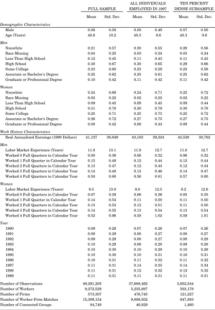
Though the underlying data are quarterly, they are aggregated to the annual level for estimation. The full sample consists of over 49 million annualized employment records on full-time workers between 25 and 65 years of age who were employed at private-sector non-agricultural …rms between 1990 and 1999.
Missing values are imputed from the posterior predictive distribution of a parametric missing data model. Speci…cs on the imputation models, and further details on sample construction and variable creation, are given in the Data Appendix to Woodcock (2005a).
Because the …xed e¤ect estimators described in Section 3.2 do not solve the least squares normal equations directly, it is possible to estimate the …xed e¤ect speci…cations on very large samples.22 Unfortunately, there currently exists no similar computational alternative to solving the mixed model equations. We must therefore estimate the mixed e¤ect speci-…cations on a subsample of observations. Sampling from linked employer-employee data is nontrivial because the sample must be su¢ciently connected to precisely estimate the person, …rm, and match e¤ects. We therefore draw a ten percent subsample of individuals employed in 1997 using the dense sampling algorithm of Woodcock (2005b). This algorithm ensures that each worker is connected to at least …ve others by a common employer, but is otherwise representative of the population of individuals employed in 1997. That is, all individuals
em-ployed in 1997 have an equal probability of being sampled.23 The dense subsample consists
22The cross-products matrix in the least squares normal equations has N +J +M +k+ 1 rows and
columns. Solving the normal equations requires inverting this matrix. This is infeasible for samples of the size considered here. Our …xed e¤ect estimates are based on the ACK conjugate gradient algorithm, which does not invert this matrix.
23The dense sampling algorithm ensures that individuals are connected to a speci…ed minimum number of
of the full work history of each sampled individual. To enable direct comparison of results between the …xed and mixed e¤ect speci…cations, we estimate the …xed e¤ect speci…cations on the full work histories of all individuals employed in 1997.
Table 1 presents characteristics of the samples. The sample of individuals employed in 1997 is largely representative of the full sample of observations. Some slight di¤erences indicate that individuals employed in 1997 have a slightly stronger labor force attachment than the sample of all individuals employed between 1990 and 1999: males are slightly over-represented, as are individuals with higher educational attainment and individuals who work four full quarters in an average calendar year. The ten percent dense subsample has characteristics virtually identical to the sample of all individuals employed in 1997.
5
Estimation Results
In discussing the empirical estimates, we focus on two comparisons. Because most prior empirical work is based on the …xed e¤ect speci…cation of the person and …rm e¤ects model, we take this as our baseline speci…cation. We compare the baseline speci…cation to mixed e¤ect estimates of the person and …rm e¤ects model. This comparison highlights the di¤er-ence between …xed and mixed e¤ect estimation methods. Our second comparison is between mixed e¤ect estimates of the person and …rm e¤ects model and mixed e¤ect estimates of the match e¤ects model. This comparison highlights the importance of match e¤ects.
Table 2 presents estimated coe¢cients ( ; ) for …xed and mixed e¤ect speci…cations of the person and …rm e¤ects model. The …xed e¤ect estimates are consistent with earlier work. The …xed e¤ect estimator produces somewhat steeper experience and education pro…les than the mixed e¤ect estimator does. We discuss this further below. The other estimated coe¢cients are very similar across speci…cations, with the exception of coe¢cients on several missing data indicators.
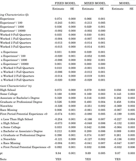
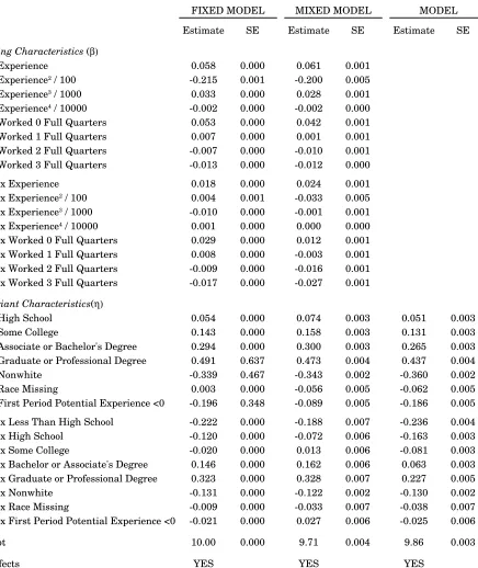
Table 3 presents estimated coe¢cients for …xed and mixed e¤ect speci…cations of the match e¤ects model. The estimated coe¢cients are broadly similar across speci…cations of the match e¤ects model, and broadly similar to the person and …rm e¤ects model. There are some notable exceptions, however. As illustrated in Figures 1 and 2, the person and …rm e¤ects model consistently over-estimates the returns to experience. For instance, …xed e¤ect estimates of the person and …rm e¤ects model imply that a male worker with 25 years of labor market experience earns 0.78 log points (118 percent) more than a labor market entrant, all
else equal. The mixed e¤ect estimator of the person and …rm e¤ects model reduces this estimate to 0.70 log points (101 percent), and introducing the match e¤ect reduces it further to 0.65 log points (92 percent). For women, the earnings di¤erential accruing to 25 years experience is 0.59 log points (80 percent) in the …xed e¤ect speci…cation of the person and …rm e¤ects model, 0.43 log points in the comparable mixed e¤ect speci…cation, and 0.39 log points (48 percent) in the mixed model with match e¤ects. The “within” estimator (12) on which the orthogonal match e¤ects and hybrid mixed e¤ect estimators are based yields an even ‡atter experience pro…le. Here, the 25 year earnings gap is 0.52 log points (68 percent) for men and 0.36 log points (43 percent) for women.24 Hence the baseline speci…cation over-estimates the returns to 25 years of experience by as much as 0.26 log points (50 percent) for men, and 0.23 log points (37 percent) for women.
Because introducing the match e¤ect ‡attens the experience pro…le so markedly, it seems that a considerable fraction of the returns traditionally attributed to labor market experience (i.e., the accumulation of general human capital) actually re‡ects the acquisition of match-speci…c human capital. A possible explanation is that individuals sort into better matches over the course of their career. When match e¤ects are omitted, the higher earnings associ-ated with sorting are attributed to labor market experience. We return to this idea below, when we investigate the sources of earnings growth when individuals change employer.
To a lesser degree, the baseline model also over-estimates the returns to education. It estimates that men with a college degree earn 0.25 log points (29 percent) more than male high-school graduates, all else equal, compared to 0.21 log points (23 percent) in the mixed model with match e¤ects. The comparable estimates are 0.29 log points (33 percent) and 0.23 log points (25 percent), respectively, for women. Here too, it seems that some of the returns traditionally associated with general human capital (education) actually re‡ect match-speci…c human capital. A possible explanation is that more educated workers sort into better matches than less educated workers. When match e¤ects are omitted, the returns to sorting into good matches are incorrectly attributed to education.
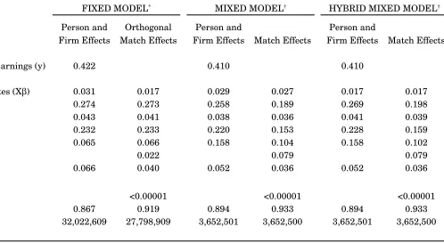
Table 4 presents the estimated variance of log earnings components. In all speci…cations, person e¤ects exhibit the greatest dispersion and the returns to time-varying characteristics exhibit the least. This is consistent with earlier estimates of the person and …rm e¤ects model, e.g., AKM, ACK, and Woodcock (2005a). The traditional mixed model and hybrid mixed model give very similar results, so we focus on results for the traditional mixed model. The …xed e¤ect estimator of the person and …rm e¤ects model exhibits the greatest dispersion in person e¤ects (0.274 squared log points) and time-varying covariates (0.031),
24Note this estimate is based entirely on within-job variation in earnings, i.e., it ignores earnings growth
and the least dispersion in …rm e¤ects (0.065). In contrast, the mixed e¤ect estimator of the person and …rm e¤ects model exhibits slightly less dispersion in person e¤ects (0.258) and time-varying covariates (0.029), and considerably more dispersion in …rm e¤ects (0.158). Introducing the match e¤ect reduces variation in the person e¤ect further (to 0.189), and reduces dispersion in the …rm e¤ect to 0.104. These imply a one standard deviation increase in the value of the person e¤ect increases log earnings by 0.435, and a one standard deviation increase in the value of the …rm e¤ect increases log earnings by 0.322. The variance of the match e¤ect itself is 0.079, so that a one standard deviation increase in the value of the match e¤ect increases earnings by 0.28 log points. This is also very substantial and nearly as large as the …rm e¤ect.
These results imply that some of the variation attributed to the match e¤ect is incorrectly attributed to person and …rm e¤ects in prior work. This not surprising, given the expres-sion we derived for the bias due to omitted match e¤ects. However, some of the variation attributed to the match e¤ect was formerly unexplained, as we see from the reduced error variance (from 0.052 to 0.036) when the match e¤ect is introduced.
The orthogonal match e¤ect estimator produces quite di¤erent results. The estimates are very similar to the person and …rm e¤ects model, with only trivial variation in the match e¤ect (0.022 squared log points). This is not surprising given the orthogonality assumption. Before proceeding further, we formally test for the presence of match e¤ects. The test is straightforward and the results are in Table 4. In the …xed model, the null hypothesis is H0 : ij = 0for each i; j pair in the data, i.e., that all match e¤ects are zero. This is a test
ofM N J = 4;176;870 linear restrictions.25 We test this hypothesis with a conventional
Wald test. Given the number of restrictions, it is no surprise that we easily reject the null of no match e¤ects at conventional signi…cance levels.26
In the mixed model speci…cations, the null of no match e¤ects isH0 : 2 = 0:We test this
hypothesis with a likelihood ratio test based on the REML log-likelihoods of speci…cations
with and without match e¤ects. Because the null hypothesis places 2 on the boundary of
the parameter space, the test statistic has a non-standard asymptotic distribution. Stram
and Lee (1994) show its asymptotic distribution is a 50:50 mixture of a 2
0 and a 21: Once
again, we easily reject the null of no match e¤ects at conventional signi…cance levels.27
25When the data consist ofGconnected groups of observations, there areN +G N J k 1 degrees
of freedom in the model without match e¤ects, andN +G M k 1 degrees of freedom in the model with match e¤ects. The model without match e¤ects therefore imposes
(N +G N J k 1) (N +G M k 1) =M N J
linearly independent restictions on the estimated e¤ects.
26The value of the Wald statistic is around 18 million.
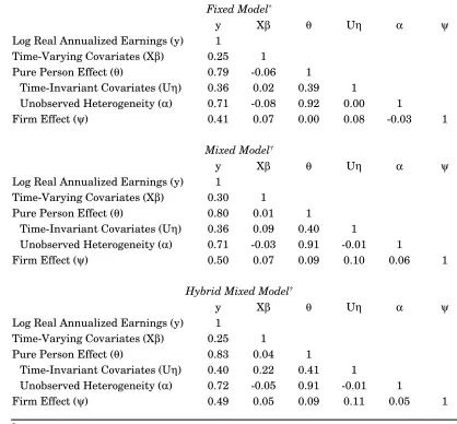
Table 5 presents sample correlations between the estimated e¤ects in the person and …rm e¤ects model. Table 6 presents the same information for the match e¤ects model. In each case, the person e¤ect is most strongly correlated with log earnings (between 0.79 and 0.89). The …rm e¤ect is also strongly correlated with log earnings: between 0.41 and 0.57, depending on speci…cation. The returns to time-varying covariates are less strongly correlated with log earnings (between 0.25 and 0.30). There is considerable variation in the estimated correlation between match e¤ects and log earnings across speci…cations. The correlation is 0.23 in the orthogonal match e¤ect speci…cation, which is comparable to the correlation between observable characteristics and log earnings. In contrast, the correlation between the match e¤ect and log earnings is around 0.60 in both mixed e¤ect speci…cations, which is second only to the correlation between the person e¤ect and log earnings.
There are several other items of note in Tables 5 and 6. One is that introducing the match e¤ect strengthens the correlation between the person e¤ect and log earnings in all speci…cations. It also strengthens the correlation between the …rm e¤ect and log earnings in both mixed e¤ect speci…cations. The match e¤ect evidently helps disentangle person-and …rm-speci…c components of log earnings. Furthermore, notice that the estimated match e¤ect is positively correlated with person and …rm e¤ects in both mixed e¤ect speci…cations. The correlation with the person e¤ect, in particular, is su¢ciently strong (0.49) that the
orthogonal match e¤ect speci…cation seems dubious.28
The correlation between person and …rm e¤ects is approximately zero in the …xed e¤ect speci…cation of the person and …rm e¤ects model and the orthogonal match e¤ects model. This is consistent with earlier estimates of the person and …rm e¤ects model based on US data (e.g., ACK and Woodcock (2005a)). Recently, Andrews et al. (2004) have argued that when the true correlation between person and …rm e¤ects is positive, the estimated correlation based on least squares estimates of the person and …rm e¤ects model is biased downward. In light of this, it is interesting to note that the correlation is noticeably larger in both mixed e¤ect speci…cations of the person and …rm e¤ects model (0.09). Introducing the match e¤ect further increases the correlation between person and …rm e¤ects by a factor of two. This suggests the bias noted by Andrews et al. (2004) is partly a characteristic of the …xed e¤ect estimator, and partly due to the omission of match e¤ects.
28The substantial correlation between person and match e¤ects might seem to contradict the assumed
5.1
Decomposing the Variance of log Earnings
The match e¤ects model de…nes a formal decomposition of the variance of log earnings into components attributable to time-varying observables, person e¤ects, …rm e¤ects, match e¤ects, and a residual component. Speci…cally,
V ar(yijt) = Cov(yijt; yijt) = Cov yijt;^ +x0ijt^ + ^i+ ^j + ^ij +eijt (24)
= Cov yijt; x0ijt^ +Cov yijt;^i +Cov yijt;^j +Cov yijt;^ij +Cov(yijt; eijt)
where ^;^i;^j;^ij are sample estimates de…ned by any of the …xed or mixed e¤ect
estima-tors, and eijt is the corresponding residual. Gruetter and Lalive (2004) present a similar
decomposition for the person and …rm e¤ects model. We have the proportional decomposi-tion:
Cov yijt; x0ijt^
V ar(yijt)
+Cov yijt; ^i V ar(yijt)
+ Cov yijt; ^
j
V ar(yijt)
+Cov yijt; ^
ij
V ar(yijt)
+Cov(yijt; eijt)
V ar(yijt)
= 1:
(25) Of course we can further decompose Cov yijt;^i =Cov(yijt;^i) +Cov(yijt; u0i^):
We present the proportional decomposition (25) in Table 7. In our baseline speci…cation, nearly 64 percent of the variance of log earnings is attributed to person e¤ects. Firm e¤ects contribute the next largest component, about 16 percent. Conditional on person and …rm e¤ects, time-varying covariates explain only 6.7 percent of the variance of log earnings, leaving more than 13 percent unexplained. Results for mixed models with person and …rm e¤ects are very similar, though both mixed e¤ect estimators attribute slightly more variation to …rm e¤ects and slightly less to person e¤ects.
5.2
Earnings Growth and Job Mobility
The match e¤ects model also provides a formal decomposition of the sources of earnings
growth when individuals change employers. For an individualiwho changes employers (from
employer j to employer n in periods t and s, respectively), the gross change in earnings is
y = yins yijt
= x0
ins x
0
ijt ^ + ^n ^j + ^in ^ij + (eins eijt)
x^ + + + e:
This de…nes a simple decomposition of earnings changes into components attributable to the change in time-varying observables, …rm e¤ects, match e¤ects, and a residual component. Again, we de…ne a proportional decomposition
x^
y + y + y +
e
y = 1 (26)
that aggregates linearly over job transitions. We use (26) to decompose the mean change in log earnings when individuals change employers into its respective components.
To decompose wage changes via (26), we focus on job-to-job transitions for two reasons. First, non-employment in the LEHD data is only identi…ed by the absence of a UI record. Periods of non-employment may therefore re‡ect unemployment, withdrawal from the la-bor force, employment not covered by the UI reporting system, or employment in a state other than the two in our sample. These may confound our ability to identify a genuine transition from one employer to another. Job-to-job transitions, which we de…ne as em-ployment spells that overlap by at least one quarter, are less subject to these confounding in‡uences. Second, job-to-job transitions are arguably more likely to violate the exogenous mobility assumption than those with an intervening period of unemployment because they are more likely to be driven by “good” and “bad” matches. Gruetter and Lalive (2004) argue this point at length. By focusing on job-to-job transitions, we can look for evidence of exogenous mobility in speci…cations with and without match e¤ects. If the proportion of earnings growth attributed to the residual component is statistically signi…cant, we take this as evidence that the exogenous mobility assumption is violated. We formalize this with the null hypothesis H0 : M1 P(eins eijt) = 0 where the summation is over all job-to-job
employment transitions, and M is the number of transitions.
increase in log earnings of 0.045 log points (0.049 in the dense subsample). Average log earnings growth in the subset of job-to-job transitions is even larger: about 0.08 log points. Of this, our baseline speci…cation attributes the largest component (about 40 percent) to time-varying covariatesX^:Firm e¤ects also contribute signi…cantly (31.6 percent). This suggests that workers ascend a “…rm ladder” when they change jobs by moving into employment at higher paying …rms. But notice that a large component of log earnings growth remains unexplained in the person and …rm e¤ects model: nearly 29 percent of log earnings growth is due to the residual component. Consequently, we easily reject the null that the residual component is zero at conventional signi…cance levels. We take this as evidence that the person and …rm e¤ects model violates the exogenous mobility assumption.
The decomposition is similar for the mixed e¤ect speci…cation of the person and …rm e¤ects model. This speci…cation attributes a larger proportion of log earnings growth to …rm e¤ects (nearly 40 percent) and a smaller proportion to the residual component (21.5 percent). Nevertheless, we still easily reject the null that the residual component is zero.
Introducing the match e¤ect overturns this result. Time-varying covariates and …rm e¤ects still contribute about equally to log earnings growth when individuals change jobs – about 40 percent each in both mixed e¤ect speci…cations. Match e¤ects explain nearly all of the remainder: about 18 percent in the mixed e¤ect speci…cations and 30 percent in the orthogonal match e¤ects speci…cation. Hence individuals sort into better matches when changing jobs, as well as into higher paying …rms. This corroborates our earlier claim that individuals sort into better matches over the course of a career, which we posited as an explanation for the biased experience e¤ect in the person and …rm e¤ects model. The substantial earnings growth accounted for by match e¤ects leaves little variation unexplained: in both mixed e¤ect models the residual component explains only about 1 percent of average growth in log earnings, and about 4 percent in the orthogonal match e¤ects speci…cation. Indeed, in both mixed e¤ect speci…cations we fail to reject the null hypothesis that the residual component is zero at the …ve percent level. We take this as evidence that the mixed e¤ect estimator of the match e¤ects model satis…es the exogenous mobility assumption.
6
Conclusion
con-tributes an additional 22 percent, and match-speci…c human capital another 16 percent. Introducing the match e¤ect helps to disentangle person and …rm-speci…c components of earnings, and corrects several biases in the person and …rm e¤ects. The person and …rm e¤ects model overestimates the returns to labor market experience and education, attributes too much variation to person e¤ects and too little to …rm e¤ects, and underestimates the correlation between person and …rm e¤ects. Taken together, these suggest that some earnings variation previously attributed to general human capital is in fact attributable to workers sorting into higher-paying …rms and better worker-…rm matches. Consequently, the person and …rm e¤ects model underestimates the implied cost of employment re-allocation over the business cycle because it understates the importance of speci…c human capital and overstates the importance of general human capital.
These biases arise because employment mobility is not exogenous conditional on observ-able characteristics, person e¤ects, and …rm e¤ects. We …nd evidence, however, that exo-geneity holds when we control for match e¤ects. Indeed, match e¤ects explain a substantial portion of the change in log earnings when individuals change employers.
References
Abowd, J. M., R. H. Creecy, and F. Kramarz (2002). Computing person and …rm e¤ects using linked longitudinal employer-employee data. Mimeo.
Abowd, J. M., F. Kramarz, and D. N. Margolis (1999). High wage workers and high wage
…rms. Econometrica 67(2), 251–334.
Abowd, J. M., P. Lengermann, and K. McKinney (2003). The measurement of human capital in the U.S. economy. Mimeo.
Abowd, J. M., B. E. Stephens, L. Vilhuber, F. Andersson, K. L. McKinney, M. Roemer, and S. D. Woodcock (2006). The LEHD infrastructure …les and the creation of the Quarterly Workforce Indicators. Technical Paper TP-2006-01, U.S. Census Bureau, LEHD and Cornell University.
Andrews, M. J., T. Schank, and R. Upward (2004). High wage workers and low wage …rms: Negative assortative matching or statistical artefact? Mimeo.
Bartel, A. P. and G. J. Borjas (1981). Wage growth and job turnover: An empirical
analysis. In S. Rosen (Ed.), Studies in Labor Markets, pp. 65–90. Chicago: National
Bureau of Economic Research.
Becker, G. S. (1964).Human Capital: A Theoretical and Empirical Analysis, with Special
Reference to Education (3rd (1993) ed.). Chicago: The University of Chicago Press.
Bureau of Labor Statistics (1997).BLS Handbook of Methods. U.S. Department of Labor.
Dostie, B. (2005). Job turnover and the returns to seniority. Journal of Business and
Economic Statistics 23(2), 192–199.
Gilmour, A. R., R. Thompson, and B. R. Cullis (1995). Average information REML: An
e¢cient algorithm for variance parameter estimation in linear mixed models.
Biomet-rics 51, 1440–1450.
Gruetter, M. and R. Lalive (2004). The importance of …rms in wage determination. IZA Discussion Paper No. 1367.
Hausman, J. A. and W. E. Taylor (1981). Panel data and unobservable individual e¤ects.
Econometrica 49(6), 1377–1398.
Henderson, C., O. Kempthorne, S. Searle, and C. V. Krosigk (1959). The estimation of
environmental and genetic trends from records subject to culling. Biometrics 15(2),
Jovanovic, B. (1979). Job matching and the theory of turnover.Journal of Political Econ-omy 87(5), 972–990.
Mincer, J. and B. Jovanovic (1981). Labor mobility and wages. In S. Rosen (Ed.),Studies in Labor Markets, pp. 21–64. Chicago: National Bureau of Economic Research.
Robinson, G. K. (1991). That BLUP is a good thing: The estimation of random e¤ects.
Statistical Science 6(1), 15–32.
Searle, S. R. (1987).Linear Models for Unbalanced Data. New York: John Wiley and Sons.
Searle, S. R., G. Casella, and C. E. McCulloch (1992). Variance Components. New York:
John Wiley and Sons.
Stevens, D. W. (2002). State UI wage records: Description, access and use. Mimeo.
Stram, D. O. and J. W. Lee (1994). Variance component testing in the longitudinal mixed
e¤ects model.Biometrics 50, 1171–1177.
Woodcock, S. D. (2005a). Heterogeneity and learning in labor markets. Mimeo.
A
Appendix: A Model of Human Capital, Wages, and
Mobility
This appendix develops a simple two-period model of wage bargaining with on-the-job search. The model illustrates several key points argued in the text regarding the relationship between match-speci…c human capital, wages, and mobility. Speci…cally, it demonstrates that when productivity depends on match-speci…c human capital, so do mobility and wages. This violates the exogenous mobility assumption of the person and …rm e¤ects model.
Workers live for two periods. In each period, they are endowed with a single indivisible unit of labor that they supply to production at home or at a …rm. Home production generates
incomeh: Workers maximize the expected present value of income.
In each period, the worker meets a …rm in a matching market. In the …rst period she meets “Firm 1,” and in the second period she meets “Firm 2.” Firms produce a homogeneous good with price normalized to one. They only produce output when matched with a worker.
The worker produces output q at Firm 1q0 at Firm 2. Both q and q0 are random variables
distributed according to F on support q; q : Productivity is unknown until the worker and
…rm meet, but is observable thereafter.
Firms maximize the net revenues from a match. For Firm 1, this is q wt where wt
denotes the period t wage payment to the worker. For Firm 2, net revenues are q0 w0
t:
Wages are determined by a Nash bargain between worker and …rm. The worker’s share of
the surplus is 2(0;1):Workers and …rms discount future income at the common rate :
The worker’s value of being employed in periodtisJt. The …rm’s value of employing the
worker is t. The …rm’s outside option is to forego production, whose value is normalized to
zero. The value of the worker’s best alternative to employment at the …rm isUt:The worker
and …rm mutually agree to engage in production if the joint surplus is non-negative, i.e., if Jt+ t Ut:In this case, the wage payment wt (or wt0) solves
max
wt
(Jt Ut) 1t : (27)
The model’s solution consists of the worker’s optimal mobility strategy and a schedule of wage o¤ers. These are summarized in the following proposition. The proof is in Appendix B.
Proposition 1 In the …rst period, the worker’s optimal strategy is to accept employment at Firm 1 if q h and remain unemployed otherwise. If she accepts employment, she is paid
w1 = q+ (1 )h+
(1 )2
2
Z q
[(2 ) (h q0
) + (q0
If the worker begins the second period unemployed, she optimally accepts employment at Firm 2 if q0 h (Case 0), and remains unemployed otherwise. If she accepts, she is paid
w0
2;C0 = q0+ (1 )h:
If the worker begins the second period employed at Firm 1, her optimal strategy is as fol-lows. If q0 h q (Case 1) she remains employed at Firm 1 and is paid w
2;C1 =
q + (1 )h: If h q0 q (Case 2), she remains employed at Firm 1 and is paid
w2;C2 = (2 ) 1[q+ (1 )q0]: Finally, if h q < q0 (Case 3), she quits
employ-ment at Firm 1 and accepts employemploy-ment at Firm 2. In this case, the wage is w0 2;C3 =
(2 ) 1[q0
+ (1 )q]:
The …rst-period wage (28) is the sum of three components: [1] the worker’s share of
output, [2] compensation for foregoing the income generated by home production, and [3] the option value of employment (the expectation term). In the proof, we show that the option value is non-positive. The intuition is simple: the worker’s second-period bargaining position is weakly improved if she is already employed at Firm 1, and she is consequently willing to accept a reduced …rst-period wage. To see this, note that the second-period wage is the bargaining-strength weighted average of match productivity and the worker’s outside option. If she begins the second period unemployed (Case 0), or if she begins the second period employed but is less productive at Firm 2 than in home production (Case 1), then
her outside option is h. When she is more productive at Firm 2 than in home production
(Cases 2 and 3), her outside option is employment at the other …rm, at a wage greater than
h: Hence employment weakly improves her second period bargaining position.
Notice the worker changes employers ifq0
> q:Hence wages and mobility both depend on productivity. If productivity depends on match-speci…c human capital, then so do wages and mobility. This violates the exogenous mobility assumption underlying the person and …rm e¤ect speci…cation (1) if the econometrician cannot observe match-speci…c human capital directly.
There are two limiting cases of this simple model that give rise to the match e¤ects model. First, normalize h to zero and let worker i’s productivity at …rmj in period t be given by
qijt=em+x
0
ijt + i+ j+ ij (29)
where m is the mean of log-productivity (common to all matches) and other terms are as
de…ned in the main text.
The …rst case arises when the worker captures the entire match surplus, so that she is
paid the value of her marginal product. That is, as ! 1 the period t wage at …rm j is
The second case is more subtle. As the di¤erence between the worker’s productivity at
Firm 1 and Firm 2 vanishes (i.e., as q0 q ! 0) the second-period wage is w
ij2 ! qij2 in
Cases 0 and 1, and wij2 !qij2 in Cases 2 and 3. Again, taking logarithms gives the match
e¤ects model.29 Furthermore, as the expected di¤erence between her productivity at Firm
1 and Firm 2 vanishes, i.e., as
(1 )3
2
Z q
0
(q0
q)dF !0;
the …rst period wage is wij1 !qij1
h
(1 )2R0qdFi. This case arises, for example, as the worker’s productivity at Firm 1 approaches the conditional mean of productivity given
xijt and i: Once again, taking logarithms gives the match e¤ects model. The option value
term, qij1 (1 )2
Rq
0 dF; will be re‡ected in the estimated returns to experience.
B
Appendix: Proofs
Proof of Proposition 1. We solve the model backward. The worker begins the second
period in one of two states. She is either unemployed or employed at Firm 1. If she is unemployed and meets Firm 2 in the matching market (Case 0), she must decide whether to remain unemployed or accept employment. ThereforeU2 =h; J2 =w20, and 02 =q0 w20:
The wage payment that solves the Nash bargain is w0
2 = q0+ (1 )h:The worker accepts
employment at Firm 2 if J2+ 02 U2; which implies q0 h:
If the worker begins the second period employed at Firm 1, she must choose between unemployment, employment at Firm 1, and employment at Firm 2. The optimal action depends onq; q0
; and h: There are three relevant subcases whereq h: We establish below
that subcases where q < h are irrelevant because the worker will not accept employment in the …rst period under these conditions.
The …rst subcase (Case 1) is q0 h q. The maximum wage that Firm 2 can o¤er is
w0
2 = q0 h: The worker prefers unemployment to employment at Firm 2, so she chooses
between unemployment and employment at Firm 1. Therefore U2 = h; J2 =w2, and 2 =
q w2:The wage payment that solves (27) isw2 = q+(1 )h:SinceJ2+ 2 =q h=U2
the worker accepts the o¤er and remains employed at Firm 1.
29The intercept di¤ers in these two cases: it isln +m in Cases 0 and 1, andm in Cases 2 and 3. Case