Is corruption anti labor?

Munich Personal RePEc Archive

Is corruption anti labor?

Roy, Suryadipta

Lawrence University

7 May 2007

Online at

https://mpra.ub.uni-muenchen.de/3199/

Is Corruption Anti Labor?

Suryadipta Roy

Lawrence University Department of Economics PO Box- 599, Appleton, WI- 54911.

Abstract

This paper investigates the effect of corruption on trade openness in low-income and high-income countries. The results suggest corruption is anti-labor, since it reduces trade in low-income countries and increases trade in high-income countries.

JEL Classification code: F0, F1, D73, C23, O17.

Keywords: Openness, corruption, Stolper-Samuelson effects.

---

Corresponding author:

Department of Economics, Lawrence University, PO Box- 599,

Appleton, WI -54911.

Email: [email protected] Phone: 920-832-7343.

1. Introduction

Global trade is beset with restrictions. These are more conspicuous in

underdeveloped countries which have higher trade protection compared to high-income

countries. A major explanation of these restrictions is that trade policies are designed at

the behest of special interest groups who benefit from such policies (e.g. Rodrik, 1995).

Recent literature has also highlighted the role of institutions in determining trade

openness and distribution of gains from openness. Anderson and Mercouiller (2004)

ascribed higher corruption and poor enforceability of contracts as important factors

limiting trade opportunities for developing countries. Given that factor proportions theory

of trade has clear distributional predictions about the effect of free trade vis-à-vis

protection, an obvious question in this context is: is effect of corruption on trade

openness any different between labor-abundant and capital-abundant countries? If

corruption is indeed anti-labor, then greater corruption would raise trade barriers in

low-income countries and reduce those in high-low-income countries, thereby adversely affecting

labor in both situations.

Marjit (2006) provides a theoretical argument on this asymmetric impact of

corruption. In his model, corruption is considered as labor-intensive activity diverting

labor away from productive activities, thereby working against the factor endowment bias

and restricting trade in labor-abundant countries. Similarly, it reinforces the relative

factor endowment bias in capital-abundant countries and hence promotes trade. Tavares

(2003) used Mayer’s (1984) median voter framework to show political rights as a proxy

for the median voter, and argued greater political rights would provide more political

corruption and political rights, (Chowdhury, 2004) greater corruption would imply

shifting of political rights away from capital-poor individuals to capitalists. This would

reduce openness in labor-abundant countries and increase openness in capital-abundant

countries. This paper sets out to test these predictions using cross-country data on

corruption, a trade policy indicator, and real percapita gross domestic product (GDP) as a

proxy for factor endowment. In the process, it (a) adds to the literature on the effect of

corruption on trade volumes across countries; and (b) comments on the income

distributional impact of corruption between labor and capital.

2. Econometric specification

Since corruption might be endogenous to trade openness, trade-GDP ratio of any

country was decomposed into exogenous measures of “natural” and “residual” openness.

This was done by estimating the expected level of openness of a country based on its

size, geographic, and linguistic characteristics using a gravity-type specification:

mmies LanguageDu i Population i moteness i GDP i import i ort + + = + )] ( log[ ) ( Re ] ) ( ) ( ) ( exp

log[ δ₁ δ₂

) (i e ummies GeographyD +

+ (1)

Wei (2000) refers to the predicted value from this regression as a country’s

exogenous “natural openness”1. The difference between actual trade-GDP ratio and this

“natural openness” captures openness determined by policy choices. This trade policy

1_{English, French, and Spanish used as language dummies. Geography dummies were a}

indicator was used as the dependent variable in the regressions. The remoteness measure

is meant to capture the impact of distance on trade. It was constructed as follows:

∑

moteness( ) ( )log[ tan ( , )]

Re , where

∑

( (2)

The following specification was used to test the main hypothesis:

it it

it t

j

it Corruption Corruption GDPpc

y =α +λ +γ +β1* +β2* *log

it

it z

GDPpc θ ε

β + +

+ ₃*log * (3)

it

y - trade policy indicator for country i in period t; α- common intercept term; λ_j and

t

γ are region-specific and time-specific effects common to all countries; βi- parameters

associated with corruption, real percapita GDP, and their interaction; - other control

variables in the regression. Countries were divided into eight regional groupings based on

Easterly (2001). These regional groupings capture effects of regional trading agreements

between countries. Use of region-specific effects also allows time-constant variables in

the two-way fixed effects regression.

z

3. Results

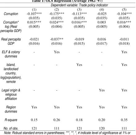
If corruption is anti-labor (or anti-poor), then in equation (3), the statistical priors

are β₁ <0 andβ₂ >0. Table 1 reports the ordinary least squares (OLS) estimates based

on cross-country means for the entire time period (1982-’97) for all variables.

International Country Risk Guide Ratings (ICRG) data were used as the corruption

measure. Both corruption and the interaction term are found to have the expected signs

and are statistically significant for the baseline specification in column (1). Thus

countries. For robustness check, other control variables were introduced in the regression.

An index of ethnolinguistic fractionalization (ELF) and colonial origins of countries

capture important structural features. Dummies for island and landlocked countries,

population size, and remoteness from other countries indicate geographical

characteristics. Legal system and religious affiliations represent cultural characteristics.

All regressions included the region dummies. The results are reported in columns (2)-(5).

In general, the main results remain quite robust and the asymmetric effect of corruption

on the trade policy indicator remains significant, except for specification (4). The effect

of percapita income on trade “policy-induced” openness seems to be sensitive to the

inclusion of the structural indicators in the presence of corruption and generally turns out

to be not significant.

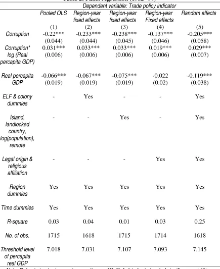
Given that cross-country averages do not capture time dimension of the

relationship, equation (3) was re-estimated as a panel. Three different panel data

estimators were considered: (a) pooled OLS; (b) two-way fixed effects; (c) random

effects regression with country-specific effects estimated by Generalized Least Squares.

The results are reported in table 2. The main hypothesis is upheld in every regression.

Inclusion of control variables does not change the basic results in any substantial way.

Percapita real GDP appears with a negative sign in all the specifications, which indicates

that trade for developed countries is mainly determined by “natural” factors rather than

policy-related issues. Indeed, percapita GDP appears to be positive and highly significant

in regressions with “natural openness” as dependent variable. The calculated threshold

level at which higher income reduces openness for different specifications is between

percapita income is found to be 7.467 indicating positive skewness in the income

distribution.

4. Other robustness checks

Other robustness checks were also conducted. Since corruption is highly

persistent for any country over time, the error terms might be serially correlated.

Following Wooldridge (2002), this was addressed by using a robust covariance matrix

adjusting for within-country correlation in the random effects regression. Moreover, since

corruption is subjective, the ICRG data might suffer from measurement error. This was

accounted for by using the Business International corruption measure used in Mauro

(1995) as proxy for the ICRG data in country average OLS regression. Since these data

come from another source, cover an earlier period (average from 1980-’83), and have

smaller country coverage (65 compared to around 120 for ICRG), measurement errors of

the two proxies are probably uncorrelated. The main results remained unchanged in both

situations2.

5. Conclusion

The basic conclusion of this paper is that an increase in corruption reduces trade

openness in low-income countries (income proxying for capital-labor ratio) and increases

openness in high-income countries. Given the median voter (generally with relatively low

labor ratio) will be pro-trade in labor-abundant countries and anti-trade in

capital-abundant countries, we can conclude that lesser corruption in low-income countries

2

should open up trade and benefit labor in those countries. A corollary to this is that

greater corruption should lead to income transfer from labor towards capitalists. It is not

far-fetched to argue that an increase in corruption would make policymakers lean more

towards the producers’ groups and enact policies in their favor in the lines of Grossman

and Helpman (2001). Thus a strong political argument can be made for improving

institutions in the developing countries since it should benefit the abundant factor in these

countries.

Appendix- Data sources

Corruption- Source: International Country Risk Guide (ICRG). Definition: Indicator of

corruption in government. Unit: 0-6, higher number denotes greater corruption.

Real per capita gross domestic product- Source: World Bank (2006). Definition:

Logarithm of real gross domestic product (GDP) divided by population. Unit: Constant

US dollars.

Trade-GDP ratio- Source: World Bank (2006). Definition: (Exports + imports)/GDP.

Unit: Percent.

Population- Source: World Bank (2006). Definition: Logarithm of population. Unit:

Absolute.

Island- Source: World Factbook 2003. Definition: Island countries indicator. Unit:

Dummy variable = 1 denoting island.

Landlocked- Source: Easterly (2001). Definition: Landlocked countries indicator. Unit:

Distance- Source: Center D’Etudes Prospectives Et D’Informations Internationales

(CEPII). Definition: Great circle distance between most populated cities. Unit:

Kilometers.

Colony- Source: CEPII. Definition: Colonial origin indicator. Unit: Dummy variables =

1 for British, French, or other colonial origin.

Fractionalization- Source: La Porta et al. (1999). Definition: Ethnolinguistic

Fractionalization, i.e. probability that any two randomly selected individuals within a

country belongs to the same religious and ethnic group. Unit: 0-1.

Legal origin- Source: La Porta et al. (1999). Definition: Dummy for origin of legal

system. Unit: Dummy variables = 1 for English, Socialist, French, German, or

Scandinavian legal origin.

Religious affiliation- Source: La Porta et al. (1999). Definition: Different religions

making up the population, divided into Protestant, Catholic, Muslim, and other

denominations. Unit: 0-1.

Region- Source: Easterly (2001). Definition: Regional groupings. Unit: Dummy

variables = 1 for East Asia & Pacific, East Europe & Central Asia, Middle East & North

Africa, South Asia, West Europe, North America, Sub-Saharan Africa, Latin America &

Caribbean regions.

References:

Anderson, J. E. and D. Marcouiller, 2002, Insecurity and the pattern of trade: an

Chowdhury, S., 2004, The effect of democracy and press freedom on corruption: an

empirical test, Economics Letters 85(1), 93-101.

Easterly, W., 2001, The lost decades: developing countries’ stagnation in spite of policy

reform 1980-1998, Journal of Economic Growth 6(2), 135-157.

Grossman, G. M. and E. Helpman, 2001, Special Interest Politics. (Cambridge and

London: MIT Press).

La Porta, R., F. Lopez-de-Silanes, A. Shleifer and R. Vishny, 1999, The quality of

government, The Journal of Law, Economics, & Organization 15(1), 222-279.

Marjit, S., 2006, Corruption, comparative advantage and missing trade, Working paper

series, City University of Hong Kong.

Mauro, P., 1995, Corruption and growth, Quarterly Journal of Economics 110(3), 681–

712.

Mayer, W., 1984, Endogenous tariff formation, American Economic Review 74(5),

970-985.

Rodrik, D., 1995, Political economy of trade policy, in: G. Grossman and K. Rogoff, eds.,

Handbook of International Economics, Vol. 3 (North-Holland: Amsterdam) 1457- 1494.

Tavares, J., 2003, Trade, factor proportions and political rights, Universidade Nova de

Lisboa, FEUNL Working paper series: 437.

Wei, S., 2000, Natural openness and good government, National Bureau of Economic

Research Working paper series: 7765.

Wooldridge, J., 2002, Econometric Analysis of Cross Section and Panel Data.

Table 1: OLS Regression (Average 1982-’97)

Dependent variable: Trade policy indicator

(1) (2) (3) (4) (5) Corruption -0.107***

(0.035) -0.175*** (0.035) -0.113*** (0.035) -0.025 (0.035) -0.104*** (0.035) Corruption* log (Real percapita GDP) 0.015*** (0.005) 0.024*** (0.004) 0.016)*** (0.005) 0.003 (0.005) 0.016*** (0.004) Real percapita GDP -0.021 (0.016) -0.037** (0.016) -0.019 (0.015) 0.016 (0.017) -0.011 (0.018)

ELF & colony dummies

- Yes - - Yes

Island, landlocked

country, log(population),

remote

- - Yes - Yes

Legal origin & religious affiliation

- - - Yes Yes

Region dummies

Yes Yes Yes Yes Yes

R-square 0.15 0.26 0.18 0.20 0.35

No. of obs. 121 111 121 120 111 Note: Robust standard errors in parentheses; ***, **, *, # indicate level of significance at 1% or

Table 2: Panel regression (1982-’97)

Dependent variable: Trade policy indicator Pooled OLS Region-year

fixed effects Region-year fixed effects Region-year Fixed effects Random effects

(1) (2) (3) (4) (5) Corruption -0.22***

(0.044) -0.233*** (0.044) -0.238*** (0.045) -0.137*** (0.046) -0.205*** (0.058) Corruption* log (Real percapita GDP) 0.031*** (0.006) 0.033*** (0.006) 0.033*** (0.006) 0.019*** (0.006) 0.029*** (0.007) Real percapita GDP -0.066*** (0.019) -0.067*** (0.019) -0.075*** (0.019) -0.022 (0.02) -0.119*** (0.038)

ELF & colony dummies

- Yes - - Yes

Island, landlocked

country, log(population),

remote

- - Yes - Yes

Legal origin & religious affiliation

- - - Yes Yes

Region dummies

Yes Yes Yes Yes Yes

Time dummies Yes Yes Yes Yes Yes

R-square 0.03 0.04 0.01 0.03 0.25

No. of obs. 1715 1618 1715 1714 1618

Threshold level of percapita

real GDP

7.018 7.031 7.107 7.093 7.145