ISSN: 1816-949X
© Medwell Journals, 2019
A New Line Search Method to Solve the Nonlinear Systems of
Monotone Equations
Karrar Habeeb Hashim, Nabiha Kahtan Dreeb, Hasan Hadi Dwail, Mohammed Maad Mahdi,
H.A. Wasi, Mushtak A.K. Shiker and Hussein Ali Hussein
Department of Mathematics, College for Pure Science, University of Babylon, Hillah, Iraq
Abstract: In this study, we suggest a new line search algorithm for solving nonlinear systems of equations such that we combine a monotone technique into a modified line search rule. The new proposed algorithm can decrease the CPU time, the number of iterations and the function evaluations and can increase the efficiency of the approach. Under some standard conditions, the global convergence of the algorithm is proved. Preliminary numerical results shows that the new algorithm is promised for solving nonlinear systems of equations monotone equations.
Key words: Nonlinear system of equations, line search method, Monotone strategy, global convergence,
numerical results, iterative method
INTRODUCTION
The nonlinear systems are one of the problems that arise in different fields of science and computational geometry, especially in the interpretation of nonlinear partial differential equations, the problem of specified value, etc. There are situations in which thousands of nonlinear equations can be solved in some independent variables effectively. Thus, finding the roots of nonlinear systems of equations has many applications in numerical and applied mathematics.
Therefore, the focus of many researchers is to find and provide appropriate ways and means to solve these non-linear systems and thus some common algorithms are suggested to solve these problem.
Nonlinear equations are one of the most important problems of multiple scientific uses such as computer science tremolo systems (Ortega and Rheinboldt, 1970; Zeidler, 2013), the first-order necessary condition for the problem of unconstrained convex optimization and also some sub-problems in generalization (Iusem and Solodov, 1997; Shiker and Sahib, 2018).
Since, the fixed points that can be found from the problem of improvement are equal to find the answer of a non-linear system of equations and the systems of nonlinear equations can be converted into problem of the lower squares this indicates a close relationship between the problems of unconstrained optimization and systems of nonlinear equations, so, it is appropriate to use unconstrained optimization algorithms to solve this problem.
One of the two important iterative methods that is used to solve nonlinear system of equations is the line search strategy, the other method is trust region. Here, we focus on the line search method and its framework. This method is fairly simple, so, its understanding and application is easy. However, they are ineffective and have some disadvantage, for example, if the array being searched for contains 30.000 items, to find the value of the last element, the algorithm will have to look at all those 30.000 elements. Typically, if we have a matrix of M elements, the linear search will identify an element in M/2 attempts. For example, if we have a matrix of 40.000 items, the linear search will compare with 20.000 items in a typical case. This is through the possibility to find the search element constantly in the array, so, the number M is always maximum in comparisons. An another disadvantage, on the large scale, the research and convergence of the line search method are slow. So, most of researchers used the monotone strategy to address that problem. Consider the nonlinear system of equations:
(1) F(x) = 0
where, F: Rn6Rn is continuous and monotone, i.e:
n F(x)-F(y), x-y 0, x, yR
By fixed point map or a natural map, some monotone variational inequality can be converted into nonlinear monotonous equations but before that there are some coercive conditions that the basic function has to achieve.
Quasi-Newton methods are considered to be one of the most important algorithms for solving problem (Eq. 1), the methods of Quasi-Newton have been a major advance in the theoretical aspect as a result of the development of solutions to many problems and this is especially, reflected in the analysis of local convergence (Broyden et al., 1973; Dennis and More, 1977). In addition, researchers have done a lot of work to create a global approximation of Quasi-Newton methods for unconstrained optimization problems see (Byrd et al., 1987; Amini et al., 2016; Nocedal, 1980 and Shiker and Amini, 2018).
By Griewank (1986) who is considered to be the closest approximation of global convergence, suggested a derivative-free line search. By Li and Fukushima (2000) had another view by constructing and deducing an example showing that the line search by Griewank (1986) contains in some special cases certain difficulties. As a result of their research and by using the non-monotonous line search method, they suggested a Gauss-Newton based BFGS method to solve nonlinear symmetric equations and a Broydens method to solve nonlinear equations also they proved these methods converge globally (Li and Fukushima, 1999, 2000). However, some of the merit functions such as the quadratic merit function are used to ensure the global approximation of Quasi-Newton.
MATERIALS AND METHODS
In this study, the new algorithm is used to solve the nonlinear monotone equations and we proved that it has a global convergence without using merit function. In comparison with BFGS method by Zhou and Li (2008) and PRP method by Cheng (2009), the new method well be more efficient. Now, we will give our algorithm.
The new algorithm (K)
Step 0. Choose an initial point x0εR n
and constants μ0 (0, 1), ρ0 (0, 1),
β0 [1/2, 1), σ0 (0, 1/2], m>0, r>0. Let k: = 0 Step 1. Compute the search direction dk by:
(2)
k k
d = -F x
Stop if dk = 0
Step 2. Determine step length αk = μ
hkβ such that h
k is the smallest
nonnegative integer h satisfies:
(3)
h h h 2
k k k k k k k
- F(x + d ), d F(x +d ) || d ||
Where k k
1+||F(z ) ||
Let zk = xk+αkdk
Stop if ||F(zk)|| = 0
Step 3. Calculate
(4)
k k k
k +1 k 2 k
k F(z ), x -z
x x - F(z )
|| F(z ) ||
Set k: = k+1 Go to Step 1.
Remark: The mapping F is Lipschitz Continuous (LC),
satisfies for a positive constant L>0 that:
(5)
n|| F x -F(y) || L || x-y ||, x, yR
It is clear that L+m>m, so:
(6)
k
kk
|| F x || || F x || || d
L+m || m
Now, we will show that the line search (3) is well-define in a similar way to Solodov and Svaiter (1998). Suppose that for some iteration index k and for any nonnegative integer h, the line search (3) is not satisfied, i.e.:
h
h
h
2
k k k k k k k
- F x +μ βd , d <ρσ μ β|| F x +βμd ||d|| *
Now if, we take limy(h64) for two side to (*):
h h
k k k k
h h
h
k k k
k k
k k k k k k k k k k k k
k k k k 2 k
2
k k
-lim F x +μ βd ,d < limρσ μ β
F x +βμd || d
- F x , d <0
- F z -αd , d <0 (since, x = z -αd
- -α F z +d , d <0
α F z +d , d <0
α F(z ) |||| d ||
)
|| | <| 0
Then, we have a contradiction, since, it is not possible to have each of αk, ||F(zk)|| and ||dk||
2 less than
zero, so, the line search is well-defined.
Convergence property: In this study, to obtain the global convergence of our algorithm then, we need the following lemma.
Lemma 1: Solodov and Svaiter (1998) let, F be monotone
and x, y0Rn satisfy +F(y), x-y,>0. Let:
+
2 F y , x-y
x = x - F(y)
Then for any x R n such that F(x)0 it holds that:
+ 2 2 + 2
|| x -x|| || x-x || -||x -x||
Now, we can state our convergence result by the following theorem similar to Solodov and Svaiter (1998).
Theorem 1: Suppose that F is LC and monotone and let
{xk} be any sequence generated by algorithm (K). Also,
we suppose that the solution set of 1 is nonempty. Then for any satisfying, x F(x)0, we have:
2 2 2
k +1 k k+1 k || x -x|| || x -x || - ||x -x ||
In particular, the sequence {xk} is bounded. Also, its satisfy that either {xk} is finite and the last iterate is a solution or the sequence is infinite and:
k +1
k k
lim||x -x ||=0
Furthermore, the sequence {xk} converges to somex
such that F(x)0.
Proof: First, if the algorithm finishes at some iteration k then: either dk = 0, so by the positive definiteness of Bk,
we get F(xk) = 0 or ||F(zk)|| = 0 in this case xk or zk will be
a solution of 1. Now suppose that dk…0 and F(xk)…0 for all
k, then:
k k k k k k k k k k k
k k k k k k k k
F z , x -z = F z , x -x - d
= F z , - d
- F z , d
= - F x + d , d
F(z )
k || k k 2 || d k || 2 >0
Then:
(7)
k k k k
k kk || k k 2 || k || 2 F z , -| |- x -z = - F z , -| |- d
F(z ) || d >0
Let be any solution of 1 andx F(x)0. From lemma 1, (4) and (12), we obtain:
(8)
2 2 2
k +1 k k+1 k || x -x|| || x -x|| -||x -x ||
In particular, the sequence{|| x -x||}k is decreasing and hence convergent. Consequently, the sequence {xk} will
be bounded and also we have:
(9) k +1 k
x
lim || x -x || 0
By Eq. 6, it is clear that {dk} holds to be bounded and
so is {zk}. From Eq. 4:
k k kk +1 k 2 k
k F z , x -z
x -x = - F(z )
|| F(z ) ||
Since, +F(zk), xk-zk, = αk+F(zk, dk, then:
x k+1 -x = k F z , -| -| d
|| F(z )|| F(z ) ( || F(z k)|| k 2||d k|| 2)/
F
k k k /
k 2 k
(z k)|| = k 2||d k|| 2
So:
(10) || x (k+1)-x k || = F(z k), -| -| x k-z k /
||F(z k)|| k 2 || d k || 2
From Eq. 9 and 10, we get:
(11)
x k K,x
lim k || d k || 0, lim k || d k|| 0
From Eq. 6, we get lim in fx64||F(xk)|| = 0, if lim in fx64 ||dk|| = 0 then by Eq. 11, we get:
(12) k
x
lim 0
Now, since, {xk} is bounded and by continuity of F,
it is clear that {xk} has some accumulation point ˆx
with F(x)ˆ 0. We also have from Eq. 8 that the sequence {|| x -x||}k ˆ converges. Therefore {xk} converges
to Eq. 3 gives us:ˆx
(13)
h h
k k-1 k k k k -1
h 2
k k-1 k k - F(x + d ), d <
F(x + d ) || d ||
Since, {xk}, {dk} are bounded, so, we can choose a subsequence, let k64 in Eq. 13, we obtain:
(14) ˆ
ˆ - F(x), d0
Such that and are limits of subsequences thatˆx dˆ
chosen. Otherwise by Eq. 6 and already familiar argument:
(15) ˆ
ˆ - F(x), d >0
k k lim in f|| F(x ) || >0
This finishes the proof.
RESULTS AND DISCUSSION
Numerical results: In this study, we compare the
performance of the new method (K) discussed earlier with the following algorithms.
PRP: It is coming from Cheng (2009).
[image:4.612.333.519.92.245.2] [image:4.612.326.517.289.444.2] [image:4.612.323.517.493.667.2]BFGS: It is coming from using the line search by Zhou and Li (2008) with the direction of this study. We wrote all the codes in MATLAB with version R2014a, also the experiments are running on a computer with 4 GB of RAM and CPU 2.30 GHz. The purpose of running the codes is to compare the results of the new algorithm (K) with the algorithms mentioned above.
When ||Fk||#10
-8 or ||F(z k)||#10
-8 or the total
number of iterates exceeds 500000 then all the algorithms will be end. In all of the algorithms, the parameters are specified as follows μ = 0.4, ρ = 0.3,
σ = 0.25, g = 10-8.
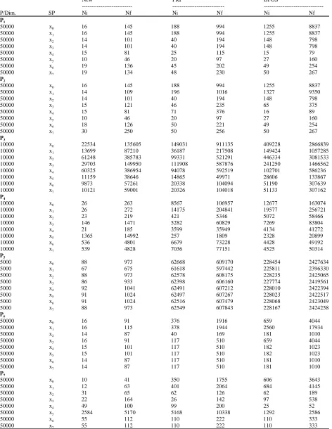
The comparison of these methods is based on three things: Ni (Number of iterations), Nf (Number of
functions evaluations) and the CPU time. Also, the special dimensions to compare these algorithms are limited to 5000|50000 for the following initial points:
T 0 1 T T 2 T 3
x (10, 10, ..., 10) , x
(-10, -10, ..., -10) , x (1, 1, ..., 1)
x (-1, -1, ..., -1)
T T 4 5 T T 6 71 2 1
x 1, , , ..., , x 0.1, 0.1, ..., 0.1 ,
2 3 n
1 2 1 2
x , , ..., 1 , x 1- , 1- , ..., 0
n n n n
Numerical results are displayed in Table 1 and 2 the first table contains both of Ni and Nf for all algorithms
while the second table contains CPU times of these algorithms.
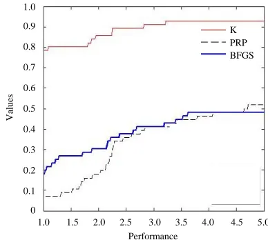
In order to obtain a comprehensive comparison of the results obtained by our proposed algorithm and the two other algorithms used in the comparison, we use the performance profile provided by Dolan and More (2002) as a tool to evaluate these algorithms and compare them through durability and efficiency (Fig. 1-3).
From the comparisons of the results we can see the superiority of the new approach compared to other
Fig. 1: Performance profile for the total number of iterations
Fig. 2: Performance profile for the total number of function evaluation
Fig. 3: Performance profile for the CPU time
methods for solving the nonlinear systems of monotone equations. Figure 1 shows the performance for the total of
No. of iterations
Va lue s K PRP BFGS
1.0 1.5 2.0 2.5 3.0 3.5 4.0 4.5 5.0 1.0 0.9 0.8 0.7 0.6 0.5 0.4 0.3 0.2 0.1 0 1.0 0.9 0.8 0.7 0.6 0.5 0.4 0.3 0.2 0.1 0
1.0 1.5 2.0 2.5 3.0 3.5 4.0 4.5 5.0 Function evaluation Va lue s K PRP BFGS 1.0 0.9 0.8 0.7 0.6 0.5 0.4 0.3 0.2 0.1 0
Table 1: Numerical results
New PRP BFGS
--- ---
---P/Dim. SP Ni Nf Ni Nf Ni Nf
P1
50000 x0 16 145 188 994 1255 8837
50000 x1 16 145 188 994 1255 8837
50000 x2 14 101 40 194 148 798
50000 x3 14 101 40 194 148 798
50000 x4 15 81 25 115 15 79
50000 x5 10 46 20 97 27 160
50000 x6 19 136 45 202 49 254
50000 x7 19 134 48 230 50 267
P2
50000 x0 16 145 188 994 1255 8837
50000 x1 14 109 196 1016 1327 9350
50000 x2 14 101 40 194 148 798
50000 x3 15 121 46 235 65 375
50000 x4 15 81 71 376 16 89
50000 x5 10 46 20 97 27 160
50000 x6 18 126 50 221 49 254
50000 x7 30 250 50 256 50 267
P3
10000 x0 22534 135605 149031 911135 409228 2866839
10000 x1 13699 87210 36187 217508 149424 1057285
10000 x2 61248 385783 99331 521291 446334 3081533
10000 x3 29703 149950 111908 587876 241250 1466562
10000 x4 60325 386954 94078 592519 102701 586236
10000 x5 11159 38646 14865 49971 28606 133867
10000 x6 9873 57261 20338 104094 51190 307639
10000 x7 10121 59001 20326 104018 51133 307162
P4
10000 x0 26 263 8567 106957 12677 163074
10000 x1 26 272 14175 204841 19577 256721
10000 x2 23 219 421 5346 5072 58466
10000 x3 146 1471 5282 60829 7269 83804
10000 x4 21 185 3599 35949 4134 41272
10000 x5 1365 14992 257 1809 2328 20899
10000 x6 536 4801 6679 73228 4428 49192
10000 x7 539 4828 7036 77151 4525 50314
P5
5000 x0 88 973 62668 609170 228454 2427634
5000 x1 67 675 61618 597442 225811 2396330
5000 x2 88 973 62578 608175 228235 2425065
5000 x3 86 933 62398 606160 227774 2419561
5000 x4 92 1041 62491 607212 228010 2422394
5000 x5 91 1024 62497 607267 228023 2422517
5000 x6 91 1024 62516 607479 228068 2423049
5000 x7 88 973 62549 607843 228167 2424258
P6
50000 x0 16 91 376 1916 659 4044
50000 x1 16 115 378 1944 2560 17934
50000 x2 14 87 40 169 181 1010
50000 x3 16 91 117 510 659 4044
50000 x4 15 101 117 510 182 1023
50000 x5 15 101 117 510 182 1023
50000 x6 14 87 117 510 181 1010
50000 x7 14 87 117 510 181 1010
P7
50000 x0 10 41 350 1755 606 3643
50000 x1 12 63 401 2064 684 4145
50000 x2 31 65 62 126 62 189
50000 x3 22 164 26 142 97 538
50000 x4 49 100 99 200 25 52
50000 x5 2584 5170 5168 10338 1292 2586
50000 x6 55 112 110 222 110 333
Table 2: Numerical results (CPU time) CPU time
---P/Dim. SP New PRP BFGS
P1
50000 x0 0.5148 4.9296 40.3730
50000 x1 0.5148 4.9608 41.4182
50000 x2 0.2652 0.7332 2.5584
50000 x3 0.3120 0.7020 2.5896
50000 x4 0.2652 0.4368 0.2652
50000 x5 0.1716 0.3744 0.5460
50000 x6 0.4212 0.7956 0.7176
50000 x7 0.3744 0.8424 0.8892
P2
50000 x0 0.5148 4.9452 42.6974
50000 x1 0.4056 5.1012 44.7410
50000 x2 0.2964 0.6708 2.8548
50000 x3 0.3588 0.8736 1.2636
50000 x4 0.2652 1.2480 0.2808
50000 x5 0.1560 0.3432 0.5304
50000 x6 0.3900 0.7956 0.7332
50000 x7 0.7488 0.9828 0.8580
P3
10000 x0 0.5265 3.6298 1.1398
10000 x1 0.3429 0.8903 0.4389
10000 x2 1.4979 2.0869 1.3758
10000 x3 0.5859 2.3832 0.5998
10000 x4 1.5049 2.3747 0.2346
10000 x5 0.1506 0.2027 0.0535
10000 x6 0.2228 0.4189 0.1233
10000 x7 0.2290 0.4198 0.1229
P4
10000 x0 0.1716 0.7960 1.0721
10000 x1 0.1716 1.5104 1.7052
10000 x2 0.1248 0.0388 0.4040
10000 x3 1.0140 0.4524 0.5508
10000 x4 0.1248 0.2664 0.2676
10000 x5 10.3116 0.0143 0.1396
10000 x6 3.2292 0.5561 0.3291
10000 x7 3.3384 0.5779 0.3325
P5
5000 x0 0.3900 2.6088 9.1360
5000 x1 0.2808 2.5382 8.9972
5000 x2 0.4056 2.6067 9.0797
5000 x3 0.3744 2.5844 9.0674
5000 x4 0.3744 2.5744 9.0594
5000 x5 0.3744 2.5384 9.0630
5000 x6 0.3744 2.5518 9.1413
5000 x7 0.3744 2.5476 9.2811
P6
50000 x0 0.5616 13.3224 0.2694
50000 x1 0.8580 13.3380 1.1963
50000 x2 0.5616 1.2012 0.0670
50000 x3 0.5616 3.6660 0.2751
50000 x4 0.7020 3.6972 0.0680
50000 x5 0.6552 3.6660 0.0656
50000 x6 0.5304 3.5256 0.0641
50000 x7 0.5772 3.6348 0.0658
P7
50000 x0 0.1560 8.4396 16.9261
50000 x1 0.2340 9.9060 18.7045
50000 x2 0.2496 0.5304 0.6708
50000 x3 0.4836 0.4836 1.7472
50000 x4 0.2808 0.9204 0.1248
50000 x5 16.8325 43.9922 8.6424
50000 x6 0.4368 0.9984 0.9672
50000 x7 0.3744 1.0608 0.9828
Ni for the three algorithms, Fig. 2 shows the performance
for the total of Nf and Fig. 3 shows the performance for the CPU time. The algorithm K solved about 95, 91 and 79% of the test functions, respectively and has least of Ni,
Nf and CPU time among the three methods and will reach
to 1 faster than the other algorithms. It means that the new algorithm K is the best algorithm closing to the performance index.
CONCLUSION
From the numerical results obtained through the comparison technique presented in the tables above of different problems with different initial points and dimensions, it is easy to conclude that the performance of the proposed algorithm K is the most efficient and effective in terms of Ni, Nf and the CPU time compared
with the two famous algorithms. This can improve the behavior of the new algorithm to solve the nonlinear monotone equations which does not require Jacobian information of the nonlinear equations. The algorithm K is able to calculate the best solution of problem (1), also its global convergence has been created without using any merit functions.
REFERENCES
Amini, K., M.A. Shiker and M. Kimiaei, 2016. A line search trust-region algorithm with nonmonotone adaptive radius for a system of nonlinear equations. 4OR, 14: 133-152.
Broyden, C.G., J.E. Dennis and J.J. More, 1973. On the local and superlinear convergence of quasi-Newton methods. IMA. J. Appl. Math., 12: 223-245. Byrd, R.H., J. Nocedal and J. Y.X Yuan, 1987.
Global convergence of a class of quasi-newton methods on Convex problems. SIAM J. Numer. Anal., 24: 1171-1190.
Cheng, W., 2009. A PRP type method for systems of monotone equations. Math. Comput. Modell., 50: 15-20.
Dennis, J.E. and J.J. More, 1977. Quasi-Newton methods, motivation and theory. SIAM Rev., 19: 46-89. Dolan, E.D. and J.J. More, 2002. Benchmarking
optimization software with performance profiles. Math. Program., 91: 201-213.
Griewank, A., 1986. The global convergence of Broyden-like methods with suitable line search. ANZIAM. J., 28: 75-92.
Li, D. and M. Fukushima, 1999. A globally and superlinearly convergent gauss-newton-based BFGS method for symmetric nonlinear equations. SIAM. J. Numer. Anal., 37: 152-172.
Li, D.H. and M. Fukushima, 2000. A derivative-free line search and global convergence of Broyden-like method for nonlinear equations. Optim. Methods Software, 13: 181-201.
Nocedal, J., 1980. Updating quasi-Newton matrices with limited storage. Math. Comput., 35: 773-782. Ortega, J.M. and W.C. Rheinboldt, 1970. Iterative
Solution of Nonlinear Equations in Several Variables. Vol. 30, Society for Industrial and Applied Mathematics, Philadelphia, Pennsylvania, USA., ISBN-13:978-0-898714-61-6, Pages: 572.
Shiker, M.A. K. and K. Amini, 2018. A new projection-based algorithm for solving a large-scale nonlinear system of monotone equations. Croatian Oper. Res. Rev., 9: 63-73.
Shiker, M.A.K. and Z. Sahib, 2018. A modified technique for solving unconstrained optimization. J. Eng. Applied Sci., 13: 9667-9671.
Solodov, M.V. and B.F. Svaiter, 1998. A Globally Convergent Inexact Newton Method for Systems of Monotone Equations. In: Reformulation: Nonsmooth, Piecewise Smooth, Semismooth and Smoothing Methods, Fukushima, M. and L. Qi (Eds.). Springer, Boston, Massachusetts, USA., ISBN: 978-1-4419-4805-2, pp: 355-369.
Zeidler, E., 2013. Nonlinear Functional Analysis and its Applications: III: Variational Methods and Optimization. Springer, Berlin, Germany, ISBN:978-1-4612-9529-7, Pages: 651.