Assessing Software Quality with Time Domain Pareto Type II using SPC

Assessing Software Quality with Time Domain Pareto

Type II using SPC

K.Sita Kumari

Associate Professor VRSEC, IT Department

Vijayawada

R Satya Prasad

Guntur

ABSTRACT

As the usage of software is getting increased day by day, there is a need for software reliability and for this several software reliability growth models exist that are capable of finding the occurrence of errors. It is also possible to find the reliability of time domain models based on order statistics with Non-Homogeneous Poisson Process (NHPP). The conditional failure rate is an important factor for software and order statistics can be used in various applications like characterization of problems, detecting outliers, linear estimation, study of system reliability, life testing, survival analysis, data compression and many others. Using Statistical Process Control (SPC), we can monitor when the software failures occurs, that helps in improving the reliability of software. In this paper, we proposed a control mechanism Pareto Type II model with an on order statistics based on NHPP and the observations are considered for time domain failure data. The unknown parameters are estimated using a well-known estimation method known as Maximum Likelihood Estimation (MLE). The model is analyzed using live data sets.

Keywords

Order Statistics, Statistical Process Control, Pareto Type II,NHPP, MLE, Control charts.

1.

INTRODUCTION

Software Reliability plays an important role in software quality. As more and more software is creeping into the embedded system, reliability has become an essential characteristic for the software. The probability that a given program will work as intended by the user without failures in a specified environment and for a specified duration can be termed as software reliability [13]. Software Reliability can prevent major faults that have the possibility of taking human life, money and time. For this a number of models have been developed for better predictions. A common approach for measuring software reliability is by using an analytical model whose parameters are generally estimated from available software failure data. Reliability quantities have been defined with respect to time, although it is possible to define them with respect to other variables. We have taken inter failures time data of Musa 1975) [ 10] and Michael [9] . In reliability study there are two characteristics of a random process: 1) the probability distribution of the random variables, i.e., Poisson and 2) the variation of the process with time. A random process whose probability distribution varies with time is called non homogeneous. The random process for time variation we can define two functions, the mean value function m(t), as the average cumulative failures associated with each time point and the failure intensity function as the rate of change of mean value function.

1.1

1.1 Statistical Process Control

Statistical Process Control (SPC) is an important tool with which we can monitor the reliability of developed software. For monitoring the software reliability, software failure data is very much essential that is available in two different types. The time domain data records the time of the failure occurrences and interval domain data records the number of failures in a given time interval. In this paper, we want to monitor the reliability of a software using SPC based on order statistics for time domain data. The main intention of this paper is to give a systematic procedure to show how SPC can be used to monitor the software reliability. In recent years, several authors have recommended the use of SPC for software process monitoring. A few others have highlighted the potential pitfalls in its use [1]. Over the years, SPC has come to be widely used among others, in manufacturing industries for the purpose of controlling and improving the quality of a product [11]. The SPC is applied in the development of software product with the intention to improve the reliability and quality of software [2]. It was proved that SPC can be applied successfully to various processes for development of software, including software reliability process. SPC is traditionally so well adopted in manufacturing industry. In general software development activities are more process centric than product centric which makes it difficult to apply SPC in a straight forward manner. The utilization of SPC for software reliability has been the subject of study of several researchers. A few of these studies are based on reliability process improvement models. They turn the search light on SPC as a means of accomplishing high process maturities. Some of the studies furnish guidelines in the use of SPC by modifying general SPC principles to suit the special requirements of software development [2](Burr and Owen[3]; Flora and Carleton[4]). It is especially noteworthy that Burr and Owen provide seminal guidelines by delineating the techniques currently in vogue for managing and controlling the reliability of software. Significantly, in doing so, their focus is on control charts as efficient and appropriate SPC tools. It is accepted on all hands that statistical process control acts as a powerful tool for bringing about improvement of quality as well as productivity of any manufacturing procedure and is particularly relevant to software development. SPC is a method of process management through application of statistical analysis, which involves and includes the defining, measuring, controlling, and improving of the processes [5].

2.

ORDER STATISTICS

variables and of functions of these variables. The use of order statistics is significant when failures are frequent or inter failure time is less. Let X denote a continuous random variable with probability density function f(x) and cumulative distribution function F(x), and let (X1 , X2 , …, Xn) denote a

random sample of size n drawn on X. The original sample observations may be unordered with respect to magnitude. A transformation is required to produce a corresponding ordered sample. Let (X(1) , X(2) , …, X(n)) denote the ordered random

sample such that X(1) < X(2) < … < X(n); then (X(1), X(2), …,

X(n)) are collectively known as the order statistics derived

from the parent X. The various distributional characteristics can be known from Balakrishnan and Cohen [7]. The inter-failure time data represent the time lapse between every two consecutive failures. On the other hand if a reasonable waiting time for failures is not a serious problem, we can group the inter-failure time data into non overlapping successive sub groups of size 4 or 5 and add the failure times with in each sub group. For instance if a data of 100 inter-failure times are available we can group them into 20 disjoint subgroups of size 5. The sum total in each subgroup would devote the time lapse between every 5th _{order statistics in a sample of size 5. In}

general for inter-failure data of size ‘n’, if r (any natural no) less than ‘n’ and preferably a factor n, we can conveniently divide the data into ‘k’ disjoint subgroups (k=n/r) and the cumulative total in each subgroup indicate the time between every rth failure. The probability distribution of such a time lapse would be that of the ordered statistics in a subgroup of size r, which would be equal to power of the distribution function of the original variable (m(t)). The whole process involves the mathematical model of the mean value function and knowledge about its parameters. If the parameters are known they can be taken as they are for the further analysis, if the parameters are not known they have to be estimated using a sample data by any admissible, efficient method of estimation. This is essential because the control limits depend on mean value function, which in turn depends on the parameters. If software failures are quite frequent keeping track of inter-failure is tedious. If failures are more frequent order statistics are preferable [5].

3.

MODEL DESCRIPTION

For calculating the parameters and the control limits using ordered Statistics approach, we consider here the Pareto Type II distribution [8].

The mean value of Pareto Type II distribution [8] representing the number of failures experienced by the time t is given by

In order to group the Time domain data into non overlapping successive sub groups of size r, we need to take m(t) to the power r

3.2 Differentiating with respect to t of equation 3.2

The Likelihood function L can be written as

Substituting equations 3.1 and 3.3 in 3.4 we get

Applying log on both sides:

Differentiating with respect to ‘a’

=>

3.6

Differentiating with respect to ‘b’

3.7

Substitute value in this equation and Differentiate with respect to ‘c’,

Taking b=1,

4.

MONITORING TIME BETWEEN

FAILURES BY DEVELOPING

CONTROL CHARTS

Several types of SPC charts are available that uses statistical techniques. It is very much important to select proper charts for implementing statistical process control based on given data, situation and need [9]. Advanced charts are also available that helps us to analyse the statistics very effectively. Variable control charts and Attribute control charts are the basic type of advanced charts that are available and can be used depending on the type of data and nature. Variable control chats are designed to control product or process parameters which are measured on a continuous measurement scale. X-bar, R charts are variable control charts. Attributes are characteristics of a process which are stated in terms of good are bad, accept or reject, etc. Attribute charts are not sensitive to variation in the process as variables charts. Forattribute data there are : p-charts, c-charts, np-charts, and u-charts. The control charts are named as Failure Control Charts that helps to assess the software failure phenomena on the basis of the given inter-failure time data.

5.

ESTIMATION OF CONTROL LIMITS

AND PARAMETERS

Parameter estimation is a statistical method trying to estimate parameters for time domain data based on ordered statistics. Given the data observations and sample size, using the equations 3.6, 3.7, 3.8, 3.9, & 3.10, the parameters ‘a’ ,’b’ and ‘c’ can be computed by using the popular Newton Rapson method . To compute the parameters a program is developed in C language .The equation for mean value function of Pareto Type II Distribution is given by

The Control limits are obtained as follows: Delete the term ‘a’ from the mean value function. Equate the remaining function successively to 0.99865, 0.00135, 0.5 and solve the value of ‘t’ , for Pareto Type II Distribution , in order to get the usual Six sigma corresponding Upper Control limit, Lower Control limit , Central line.

F(t)=

=0.99865 =1-0.99865

=0.00135

= Apply log on both sides

The control limits are defined in such a way that the point above the ) (5.1) Upper Control Limit (UCL) is an alarm

better. A point within the control limits indicates that the process is stable.

5.1

Developing Failure Charts

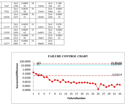
Given the n inter-failure data the values of m(t) at , , and at the given n inter-failure times are calculated. Then successive differences of the m(t)’s are taken, which leads to n-1 values. The graph with the said inter-failure times 1 to n-1 on X-axis, the n-1 values of successive differences m(t)’s on Y-axis, and the 3 control lines parallel to X-axis at m( ), m( ), m( ) respectively constitutes failures control chart to assess the software failure phenomena on the basis of the given inter-failures time data.

6.

ILLUSTRATION

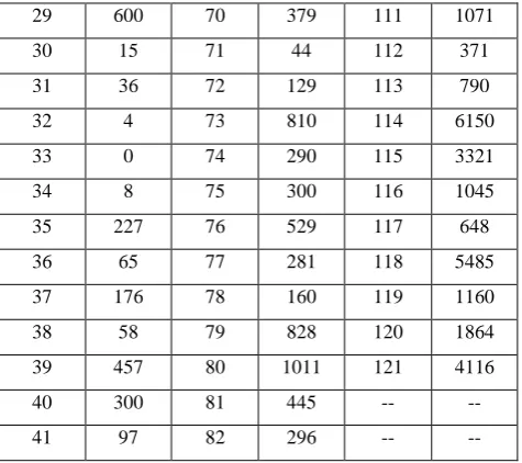
The procedure of generating the failures control charts for failure software process is illustrated considering the live data sets [9][10]. The results have given the +ve recommendations that software reliability can be assessed and the failures are detected at an early stage.

Table 1: Software failure data reported by Musa(1975) [10]

Fault Time Fault Time Fault Time

1 3 42 263 83 1800

2 30 43 452 84 865

3 113 44 255 85 1435

4 81 45 197 86 30

5 115 46 193 87 143

6 9 47 6 88 108

7 2 48 79 89 0

8 91 49 816 90 3110

9 112 50 1351 91 1247

10 15 51 148 92 943

11 138 52 21 93 700

12 50 53 233 94 875

13 77 54 134 95 245

14 24 55 357 96 729

15 108 56 193 97 1897

16 88 57 236 98 447

17 670 58 31 99 386

18 120 59 369 100 446

19 26 60 748 101 122

20 114 61 0 102 990

21 325 62 232 103 948

22 55 63 330 104 1082

23 242 64 365 105 22

24 68 65 1222 106 75

25 422 66 543 107 482

26 180 67 10 108 5509

27 10 68 16 109 100

28 1146 69 529 110 10

29 600 70 379 111 1071

30 15 71 44 112 371

31 36 72 129 113 790

32 4 73 810 114 6150

33 0 74 290 115 3321

34 8 75 300 116 1045

35 227 76 529 117 648

36 65 77 281 118 5485

37 176 78 160 119 1160

38 58 79 828 120 1864

39 457 80 1011 121 4116

40 300 81 445 -- --

41 97 82 296 -- --

Table: 2 Parameter estimates and their control limits of 4

and 5 order

Data

Set Or

der

a b c m(

) m( ) m( ) Mus a

4 26.0 268 1.00 028 3.96 197 25.9 916 13.0 134 0.03 514 5 27.0

071 1.00 011 4.47 055 26.9 707 13.5 036 0.03 646

Table: 3 Successive differences of 4th order m(t)’s of

Table 1 Fa ult 4-order Cumul atives

m(t) Succes

sive Differ ence’s Of m(t)’s Fa ult 4-order Cumul atives

m(t) Succes

UCL 25.99160

CL 13.01340

LCL 0.03514

0.0000 0.0001 0.0010 0.0100 0.1000 1.0000 10.0000 100.0000

1 3 5 7 9 11 13 15 17 19 21 23 25 27 29 31 33

Su

cc

e

ssi

ve

D

iff

e

re

n

ce

FailureNumber FAILURE CONTROL CHART

11 7447

26.0 1296

0.0008 29

28

52042 26.0 248

5.18E-05 12

7922 26.0 1379

0.0029 58

29

53443 26.0 2486

0.0001 04 13

10258 26.0 1675

0.0008 23

30

56485 26.0 2496

0.0001 79

14

11175 26.0 1757

0.0010 15

31

62651 26.0 2514

5.67E-05 15

12559 26.0 1859

0.0005 63

32

64893 26.0 252

0.0002 33 16

13486 26.0 1915

0.0008 95

33

76057 26.0 2543

0.0001 93 17

15277 26.0 2005

0.0004 45

34

88682 26.0 2562

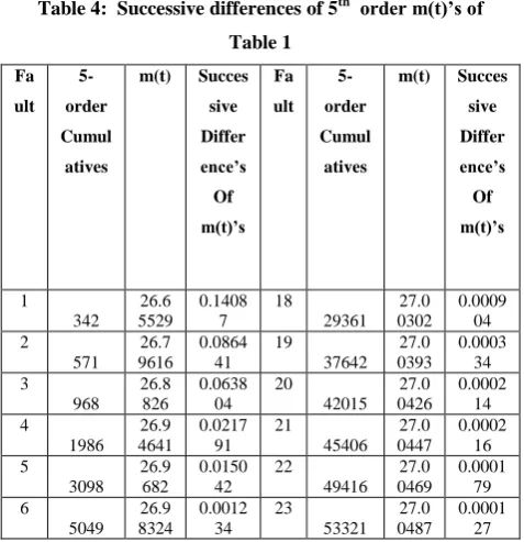
Table 4: Successive differences of 5th order m(t)’s of Table 1 Fa ult 5-order Cumul atives

m(t) Succes

sive Differ ence’s Of m(t)’s Fa ult 5-order Cumul atives

m(t) Succes

sive Differ ence’s Of m(t)’s 1 342 26.6 5529 0.1408 7 18 29361 27.0 0302 0.0009 04 2 571 26.7 9616 0.0864 41 19 37642 27.0 0393 0.0003 34 3 968 26.8 826 0.0638 04 20 42015 27.0 0426 0.0002 14 4 1986 26.9 4641 0.0217 91 21 45406 27.0 0447 0.0002 16 5 3098 26.9 682 0.0150 42 22 49416 27.0 0469 0.0001 79 6 5049 26.9 8324 0.0012 34 23 53321 27.0 0487 0.0001 27 7 5324 26.9 8447 0.0037 5 24 56485 27.0 0499 0.0002 1 8 6380 26.9 8822 0.0031 26 25 62661 27.0 0521 0.0003 03 9 7644 26.9 9135 0.0038 24 26 74364 27.0 0551 0.0001 96 10 10089 26.9 9517 0.0009 72 27 84566 27.0 057 -0.0008 9 11 10982 26.9 9615 0.0013 79 28 52042 27.0 0481 6.08E-05 12 12559 26.9 9753 0.0014 03 29 53443 27.0 0487 0.0001 22 13 14708 26.9 9893 0.0007 48 30 56485 27.0 0499 0.0002 1 14 16185 26.9 9968 0.0006 6 31 62651 27.0 052 6.65E-05 15 17758 27.0 0034 0.0009 28 32 64893 27.0 0527 0.0002 73 16 20567 27.0 0127 0.0012 09 33 76057 27.0 0554 0.0002 26 17 25910 27.0 0247 0.0005 47 34 88682 27.0 0577

Fig 2 : Failure Control chart of Table 4

UCL 26.97070

CL 13.50360

LCL 0.03646

0.0000 0.0001 0.0010 0.0100 0.1000 1.0000 10.0000 100.0000

1 3 5 7 9 11 13 15 17 19 21 23 25 27 29 31 33

7.

CONCLUSION

The Failure control charts of Figure 1 and Figure 2 have shown out of control signals i.e., below LCL. . By observing Failure Control Charts, it is identified that failures are detected at early stages. The early detection of software failure will considerably improve the software reliability. Hence our method of estimation with order statistics and the control charts are giving a +ve recommendation for their use in monitoring the reliability of a software.

8.

REFERENCES

[1]. N. Boffoli, G. Bruno, D. Cavivano, G. Mastelloni; Statistical process control for Software: a systematic approach; 2008 ACM 978-1-595933-971-5/08/10. [2]. K. U. Sargut, O. Demirors; Utilization of statistical

process control (SPC) in emergent software organizations: Pitfallsand suggestions; Springer Science + Business media Inc. 2006

[3] Burr,A. and Owen ,M.1996. Statistical Methods for Software quality . Thomson publishing Company. ISBN 1-85032-171-X.

[4] Carleton, A.D. and Florac, A.W. 1999. Statistically controlling the Software process. The 99 SEI Software Engineering Symposimn, Software Engineering Institute, Carnegie Mellon University

[5]. K.Ramchand H Rao, R.Satya Prasad, R.R.L.Kantham; Assessing Software Reliability Using SPC – An Order Statistics Approach; IJCSEA Vol.1, No.4, August 2011

[6] Arak M. Mathai ;Order Statistics from a Logistic Dstribution and Applications to Survival and Reliability Analysis;IEEE Transactions on Reliability, vol.52, No.2; 2003

[7] Balakrishnan.N., Clifford Cohen; Order Statistics and Inference; Academic Press inc.;1991

[8] R.Satya Prasad, K.Sita kumari, G.Sridevi; Assessing pareto software reliability using SPC, IJCSI, Vol 10, Issue 1, January 2013

[9] Ronald P.Anjard;SPC CHART selection process;Pergaman 0026-27(1995)00119-0Elsevier science ltd.

[10] R.SatyaPrasad, “ Software Reliability with SPC”; International Journal of Computer Science and Emerging Technologies; Vol 2, issue 2, April 2011. 233-237 [11] M.Xie, T.N. Goh, P. Rajan; Some effective control chart

procedures for reliability monitoring; Elsevier science Ltd, Reliability Engineering and system safety 77(2002) 143- 150

[12]. R Satya Prasad, N Geetha Rani,“Pareto type II software reliability growth model”, International Journal of Software Engineering, Vol. 2, Issue 4, 2011. pp. 81-86 [13] Pham. H., 2003. “Handbook of Reliability Engineering”,