Closed Form Solution of Nonlinear Quadratic Optimal Control Problem by State control Parameterization using Chebyshev Polynomials

Closed Form Solution of Nonlinear-Quadratic Optimal

Control Problem by State-Control Parameterization

using Chebyshev Polynomials

Hussein Jaddu

Al Quds University

P.O.Box 20002 Abu Dies, Jerusalem, Palestine

Milan Vlach

School of Mathematics and Physics Charles University

Malostranske namesti 25, 11800 Praha 1, Czech Republic

ABSTRACT

In this paper the quasilinearization technique along with the Chebyshev polynomials of the first type are used to solve the nonlinear-quadratic optimal control problem with terminal state constraints. The quasilinearization is used to convert the nonlinear quadratic optimal control problem into sequence of linear quadratic optimal control problems. Then by approximating the state and control variables using Chebyshev polynomials, the optimal control problem can be approximated by a sequence of quadratic programming problems. The paper presents a closed form solution that relates the parameters of each of the quadratic programming problems to the original problem parameters. To illustrate the numerical behavior of the proposed method, the solution of the Van der Pol oscillator problem with and without terminal state constraints is presented.

General Terms:

Control Systems, Numerical Method

Keywords:

Nonlinear optimal control problem, Chebyshev polynomials, Quasilinearization, Iterative method

1. INTRODUCTION

Optimal control problems can be solved using the direct method by employing either the discretization technique or the parameterization technique [1-8]. There is a number of research papers which describe the use of the parameterization technique. Some accomplish parameterization by approximating the control variables by a function of unknown parameters [2], some by approximating the state variables [5-6,9] and some by approximating both the state and the control variables [3-4,7,10-11] .

In [10], a method to solve a nonlinear optimal control problem by approximating the state and control variables by Chebyshev series has been proposed. The method converts the nonlinear optimal control problem into a nonlinear mathematical programming problem. The proposed method, however, is complicated in approximating the state equations and the performance index.

In [12], Jaddu presented a method to solve the constrained linear optimal control problem using state-control parameterization. Also in [8], a closed form solution of the linear quadratic optimal control problem was proposed. In this paper, the method of [12] and the work of [8] are extended to obtain a closed form solution of a nonlinear optimal control problem subject to initial and terminal state constraints. The proposed method is based on using the quasilinearization, therefore, the original nonlinear optimal control problem is approximated by a sequence of time-varying linear-quadratic optimal control problems. Then each of the state variables and control variables is approximated by a finite length Chebyshev series of unknown parameters. In this way the original nonlinear optimal control problem is converted into a sequence of quadratic programming problems. The use of the quasilinearization enables us to express the quadratic programming problems’ parameters in terms of the parameters of the original problem, which simplifies the implementation of the method. The method approximates the state equations and the performance index in a different and easier way in comparison with the method of [10]. To illustrate the effectiveness of the proposed algorithm, the results of solving Van der Pol oscillator optimal control problem with and without terminal state constraints are presented.

2. PROBLEM STATEMENT

The system whose behaviour is described by the following system of differential equations is considered

˙

x=f(t,x,u) 0≤t≤tf (1) wheretf is a fixed terminal time;xis ann×1state vector,uis anm×1control vector;f : Rn_×Rm _{→ R}n_{is continuously} differentiable with respect to its arguments.

The initial condition of the system is:

x(0) =x0 (2)

and the terminal state constraints are given by: x(tf)∈ S

whereSis a given nonempty subset ofRn_{. The following case is} treated in this paper

S={x∈Rn_|Ex(t

whereEis ans×nconstant matrix,xf is a givens×1vector of terminal conditions. However, the method is equally suitable for

S=Rn_{, that is, for problems with no terminal constraints.} As a set of feasible controls, take the set U consisting of all piece-wise continuous functionu: [0, tf]→Rmfor which there exists a solution of (1) such that (2) and (3) are satisfied.

The problem is to find a feasible control that minimizes, over the set of all feasible controls, the quadratic performance indexJ :U →

R1_{given by:}

J(u) = Z tf

0

(xTQx+uTRu)dt (4)

whereQis ann×n positive semidefinite matrix, andRis an m×mpositive definite matrix.

3. PROBLEM REFORMULATION

To solve the problem of the previous section, the second method of the quasilinearization is applied [13]. The performance index is expanded up to the second order and the constraints are expanded up to the first order around a nominal state vector xk_{(t) and a} nominal control vectoruk_(t).

The quasilinearization replaces the nonlinear optimal control problem (1)-(4) by a sequence of time-varying linear-quadratic optimal control problems given, for each k = 0,1,2,· · ·, as follows:

Minimize:

Jk+1_(uk+1_{) =}

Z tf

0

((xk+1₎T_Qxk+1_+(uk+1₎T_Ruk+1_{)dt (5)}

subject to the linearized state equations, initial conditions and terminal state constraints given by:

˙

xk+1 = Ak(t)xk+1+Bk(t)uk+1+hk(t) (6)

xk+1(0) = x0 (7)

Exk+1(tf) = xf (8)

where:

hk_{(t) = f(t,x}(k)_,u(k)_)−Ak_(t)x(k)_−Bk_(t)u(k)

Ak_{(t) =} ∂f(t,x,u) ∂x

_xk,uk

Bk(t) = ∂f(t,x,u) ∂u

xk_,uk

The next step in the proposed method is to convert each of the linear quadratic optimal control problems (5)-(8) into a quadratic programming problem by approximating each of the state variables and control variables by finite length Chebyshev polynomials of unknown parameters. The time intervalt∈ [0, tf]of the optimal control problem has to be changed to τ ∈ [−1,1] because Chebyshev polynomials are orthogonal on this range. In the new settingτ =−1is the initial time andτ = 1is the terminal time. Expressing the problem (5)-(8) in terms ofτ, gives

Jk+1(uk+1) = tf 2

Z 1

−1

((xk+1)TQxk+1+ (uk+1)TRuk+1)dτ (9) subject to the constraints given by:

2 tf

dxk+1_(τ)

dτ = A

k_(τ)xk+1_+Bk_(τ)uk+1_+hk_(τ) (10)

xk+1_{(−1) = x}

0 (11)

Exk+1_{(1) = x}

f (12)

Expanding each of the state variables xk+1_{(τ) and the control}

variablesuk+1_{(τ)by a Chebyshev series of orderN, results in}

xk_j+1(τ) = N X

i=0

aj_i(k+ 1)Ti(τ) j= 1,2,· · ·, n (13)

uk+1

r (τ) = N X

i=0

br

i(k+ 1)Ti(τ) r= 1,2,· · ·, m (14)

whereaj_i(k+ 1)s andbr

i(k+ 1)s are(N+ 1)nand(N+ 1)m unknown parameters respectively; Ti(τ) is the i-th Chebyshev polynomial.

These two systems of equations can be rewritten using the Kronecker product⊗[14] as follows:

xk+1(τ) = (TT(τ)⊗In)ak+1 (15)

uk+1(τ) = (TT(τ)⊗Im)bk+1 (16)

where: aTk+1 = [a

1

0(k+ 1)a 2

0(k+ 1)· · ·a

n

0(k+ 1)a 1

1(k+ 1)· · ·

an

1(k+ 1)· · ·anN(k+ 1)] bT

k+1 = [b10(k+ 1)b20(k+ 1)· · ·bm0(k+ 1)b11(k+ 1)· · ·

bm

1 (k+ 1)· · ·b

m N(k+ 1)] TT_{(τ) = [T}

0(τ)T1(τ) · · · TN(τ)]

andIn,Imaren×nandm×midentity matrices respectively.

3.1 Performance Index Approximation

Substituting (15) and (16) into (9), gives:

Jk+1

N (ak+1,bk+1) =

tf 2

Z 1

−1

aT

k+1(T⊗In)Q(TT⊗In)ak+1+

bT

k+1(T⊗Im)R(TT⊗Im)bk+1dτ (17)

where the values of J_Nk+1 are the approximate values of Jk+1

obtained through approximation of the state and control variables by N-th order Chebyshev series. This equation can be simplified to:

J_Nk+1(ak+1,bk+1) =

tf 2

Z 1

−1

(aT k+1(TT

T_⊗Q)a k+1+

bT k+1(TT

T_⊗R)b

k+1)dτ (18)

which can be written in compact form as: Jk+1

N (zk+1) =

1 2z

T

k+1Hzk+1 (19)

where: zT

k+1 =

aT

k+1 b

T k+1

H = tf Z 1

−1

TTT_{⊗Q O}

OT _TTT_⊗R

dτ

3.2 Constraints Approximation

To approximate the state equation, the initial condition and the terminal state constraints, equation (13) is written as follows:

xk+1= N X

i=0

Tiαi(k+ 1) (20)

or:

xk+1 _{= T}T_[αT

0(k+ 1)α

T

1(k+ 1)· · ·α

T N(k+ 1)]

T

= TT_α

k+1 (21)

where: αT

i(k+ 1) =

a1

i(k+ 1) a

2

i(k+ 1) · · · a n i(k+ 1)

Similarly, the control variables (14) can be written as:

uk+1 _{= T}T_[βT

0(k+ 1)β

T

1(k+ 1) · · ·β

T N(k+ 1)]

T

= TT_β

k+1 (22)

where: βT

i(k+ 1) =

b1

i(k+ 1) b2i(k+ 1) · · · bmi (k+ 1)

Notice that αk+1 = ak+1 and βk+1 = bk+1. However,

the multiplication in equations (21) and (22) has to take place block-wise, while the multiplication in equations (15) and (16) is performed element-wise.

Also,Ak_{(τ), B}k_(τ)andhk_{(τ)have to be expanded by a finite} Chebyshev series.

The approximation ofAk_{(τ)can be given by:}

Ak_{(τ) =} N X

i=0

AiTi

= [A0A1 · · ·AN]T (23)

whereAi, i = 0,1,· · ·N is an n×n constant matrix of the coefficient of the Chebyshev polynomialTi.Ai’s can be obtained as follows [15]:

A0 =

1 M

M X n=1

A(cos(θn))

Ai = 2 M

M X n=1

A(cos(θn))cos(iθn) i= 1,2,· · ·, N

whereθn=2₂n_M−1π, n= 1,2,· · ·, MandM > N.

Similarly,Bk_{(τ)can be expanded by Chebyshev series and can be} expressed as:

Bk(τ) = [B0B1 · · · BN]T (24) whereBiis ann×mmatrix of constant elements.

Following the same procedure the vectorhk_{(τ)can be expanded} into a Chebyshev series as:

hk(τ) = TT[hT0 h

T

1 · · ·h

T N]

T

= TTH (25)

where:

hTi =

h1

i h2i · · · hni

Notice that the multiplications in (23), (24) and (25) is performed block-wise.

The last part of the state equation (10) to be approximated isx˙k+1_,

which can be expressed in terms of the parameters ofxk+1_{. This}

can be achieved, by using the differentiation operational matrixD [16] given in the appendix, as follows:

˙

xk+1_{(τ) =T}T_DT_α

k+1 (26)

Substituting (21), (22), (23), (24), (25) and (26) into (10), gives 2

tf

TT_DT_α

k+1 = [A0· · ·AN]TTTαk+1+

[B0· · ·BN]TTTβk+1+TTH (27)

The right hand side can be simplified using the property of Chebyshev polynomials derived in [17]. Although this property is derived for the Chebyshev polynomials of the second type, it can be proved that the same property holds for the Chebyshev polynomials of the first type that are used in this work. Applying this property yields,

A0A1 · · ·ANTTT = TTA (28)

B0B1 · · · BN

TTT _{= T}T_B

(29) whereA,Bare constant matrices given in the appendix.

Substituting (28) and (29) into (27) gives: 2

tf

TT_DT_α

k+1=TTAαk+1+TTBβk+1+TTH (30)

In this equation the multiplications have to be performed block-wise. To be able to perform element-wise multiplication, this equation can be rewritten as:

2 tf

(TT_DT_⊗I

n)αk+1 = (TT⊗In)Aαk+1+

(TT⊗In)Bβk+1+ (TT⊗In)H (31) Using the Kronecker product properties [14], this equation can written as:

2 tf

(TT_⊗I

n)(DT⊗In)αk+1 = (TT⊗In)Aαk+1+

(TT⊗In)Bβk+1+ (TT⊗In)H (32) Equating the coefficients ofTT_⊗I

non both sides, yields: 2

tf

(DT⊗In)αk+1=Aαk+1+Bβk+1+H (33)

In this equationαk+1andβk+1can be replaced byak+1andbk+1

respectively to become:

(A − 2

tf

(DT⊗In))ak+1+Bbk+1+H= 0 (34)

This equation will replace the system state equation (10).

In addition to the state equations, the initial conditions and the terminal state constraints have to be approximated. Substituting (15) into both (11) and (12), yields:

(TT_(−1)⊗I

n)ak+1=x0 (35)

E(TT_(1)⊗I

Combining equations (35),(36) with (34), yields: 



A − 2

tf(D

T_⊗I n) TT_(−1)⊗I

n E(TT_(1)⊗I

n)  ak+1+

" _B O(n×m(N+1))

O(s×m(N+1))

# bk+1+

" _H

−x0

−xf #

= 0 (37)

or  

A − 2

tf(D

T_⊗I

n) B TT_(−1)⊗I

n O(n×m(N+1))

E(TT_(1)⊗I

n) O(s×m(N+1))



zk+1= ˜h (38)

where

zk+1=

ak+1

bk+1

˜ h=

"_−H x0

xf #

Equation (38) represent the equality constraints that replace the state equations, initial condition and the terminal state constraints. Each of the time-varying linear-quadratic optimal control problems (5)-(8) is converted into a quadratic programming problem. The new problem is to find a vectorz∗

k+1that minimizes:

J_Nk+1(zk+1) =

1 2z

T

k+1Hzk+1 (39)

subject to:

Fzk+1= ˜h (40)

where:

F=

"_{A −} 2

tf(D

T_⊗I

n) B T(−1)⊗In O(n×m(N+1))

ET(1)⊗In O(s×m(N+1))

#

Thenstate equations are replaced byn(N+1)equality constraints while the initial condition and the terminal state constraints represent an additionaln+sequality constraints. Hence each of the linear quadratic optimal control problems (9)- (12) is approximated by quadratic programming problem of(n+m)(N+ 1)unknown parameters andn(N+ 2) +sequality constraints. Therefore, to make sure that the number of the unknown parameters is greater than the number of equality constraints, the following inequality should hold when choosing the orderNof the approximation:

N >n+s−m

m (41)

The solution of the quadratic programming problem can be obtained by matrix-vector multiplication and the optimal value of the unknown parameters vectorzis given by:

z∗_k+1=H−1_FT_(FH−1_FT₎−1_{h˜ (42)}

After obtaining the optimal value of the unknown parameters vector, these values will be substituted back into equations (13) and (14) to obtain the new nominal state vector and the new nominal control vector that will be used to obtain the next linear quadratic optimal control problem. This process is continued until

|J_Nk+1−Jk

N|is small enough. In this work the computations are terminated when|J_Nk+1−Jk

N| ≤1×10

−4_.

In order to decide whether the computed solution is close enough to the optimal solution, the following criteria is used: Substitution of the calculated controluk_{(t)of the last iteration into the state} equation (1) gives:

˙

x=f(t,x(t),uk(t)) (43) Numerical integration of (43) is possible for a given initial or final conditions. Ifˆx(t)is the solution of the numerical integration, then the following criteria can be used to estimate the error

dyn= max

0≤t≤t_f|ˆx(t)−x k_(t)|

(44)

4. NUMERICAL EXAMPLE

To illustrate the numerical behaviour of the proposed method, the Van der Pol oscillator problem is considered. The problem is to minimize the performance index:

J= Z 5

0

(x21+x 2 2+u

2

)dt (45)

subject to the state equations and initial conditions given by: ˙

x1 = x2 (46)

˙

x2 = −x1+x2−x21x2+u (47)

x1(0) = 1andx2(0) = 0,

Applying the quasilinearization and expressing the problem in terms ofτ, the following sequence of problems is obtained: For k= 0,1,2· · ·, minimize:

Jk+1₌5

2 Z 1

−1

(xk+1

1 )

2_{+ (x}k+1 2 )

2_{+ (u}k+1₎2

dτ (48)

subject to the linearized state equations and initial conditions: 2

5 "

dxk₁+1 dτ dxk₂+1

dτ #

=

0 1

−1−2xk

1xk2 1−xk1 2 x

k+1 1

xk2+1

+

0 1

uk+1

+

0 2xk

1 2

xk

2

xk₁+1(−1) = 1 xk2+1(−1) = 0

This problem is solved using the proposed algorithm, starting from x0

1 = x02 = 0and expanding each of the state variables and the

The optimal states and the optimal control forN = 11are shown in Fig. 1 and Fig. 2 respectively.

0 0.5 1 1.5 2 2.5 3 3.5 4 4.5 5

−0.6 −0.4 −0.2 0 0.2 0.4 0.6 0.8 1

Time

State x(t)

x1

x2

Fig. 1. Optimal state x(t) for unconstrained case

0 0.5 1 1.5 2 2.5 3 3.5 4 4.5 5

−0.6 −0.4 −0.2 0 0.2 0.4 0.6 0.8 1 1.2

Time

Control u(t)

Fig. 2. Optimal control u(t) for unconstrained case

Also, the previous problem is solved, but with the following terminal state constraints:

x1(5) = −0.97

x2(5) = −0.96

forN = 5, N = 7, N = 9andN = 11. The case,N = 3is excluded because it does not satisfy the condition of (41). The approximate optimal values along with their differences in subsequent iterations and the error estimatedynare summarized in Table 2. The initial and the terminal state constraints are exactly

satisfied. The optimal states and control forN = 11are shown in Fig. 3 and Fig. 4 respectively.

0 0.5 1 1.5 2 2.5 3 3.5 4 4.5 5

−1 −0.8 −0.6 −0.4 −0.2 0 0.2 0.4 0.6 0.8 1

Time

State x(t)

x1

x2

Fig. 3. Optimal state x(t) for constrained case

0 0.5 1 1.5 2 2.5 3 3.5 4 4.5 5

−0.6 −0.4 −0.2 0 0.2 0.4 0.6 0.8 1 1.2

Time

Control u(t)

Fig. 4. Optimal control u(t) for constrained case

The problem with terminal state constraints was solved by Frick and Stech [11] using Epsilon-Ritz method on parallel processor array. They found an approximate optimal value to be4.2490in five iterations.

Table 1. Approximate optimal value for the first case

N k J_Nk+1 |J_Nk+1−Jk

N| dyn

N=3 0 4.02168387 –

1 3.53249140 0.489192

2 3.52811178 0.004379

3 3.52827537 0.000163

4 3.52826923 0.000006 0.38

N=5 0 3.38355087 –

1 2.86896807 0.514580

2 2.86865514 0.000131

3 2.86867141 0.000016 0.032

N=7 0 3.37167025 –

1 2.86798210 0.503688

2 2.86789913 0.000082 1.8×10−3

N = 9 0 3.37164338 –

1 2.86693354 0.504709

2 2.86703264 0.000099 6×10−4

N=11 0 3.37164327 –

1 2.86685508 0.504788

2 2.86695986 0.000104

3 2.86695565 0.000004 7.3×10−5

Table 2. Approximate optimal value for the second case

N k J_Nk+1 |J_Nk+1−Jk

N| dyn

N=5 0 4.49271577 –

1 4.24763913 0.245076

2 4.24842816 0.000789

3 4.24833707 0.000091 0.033

N=7 0 4.49107754 –

1 4.22138666 0.269690

2 4.22217961 0.000792

3 4.22219794 0.000018 6.1×10−3

N=9 0 4.49100236 –

1 4.22037466 0.270627

2 4.22015874 0.000215

3 4.22016087 0.000002 0.83×10−3

N=11 0 4.49100235 –

1 4.22023610 0 .270766

2 4.22004433 0.000191

3 4.22004500 0.0000006 1.2×10−4

Table 3. Difference betweenJ2

NandJ

3

N

unconstrained case constrained case

N |J2

N−J

3

N| N |J

2

N−J

3

N|

3 0.000163

5 0.000016 5 0.000091

7 0.000003 7 0.000018

9 0.000007 9 0.000002

11 0.000004 11 0.0000006

5. CONCLUSION

A computational method is proposed to solve the nonlinear quadratic optimal control problem with initial and terminal state constraints. The method reduces the problem into solving sequence of quadratic programming problems which can be solved easily by matrix vector multiplications. The sequence of the approximate optimal values generated by the method seems to converge very fast to the optimal value. It is believe that this is due to the use of quasilinearization and the use of Chebyshev polynomials.

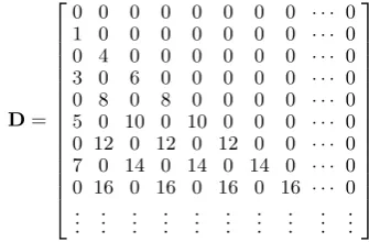
6. APPENDIX

Chebyshev polynomials’ differentiation operational matrixD[16] is given by:

D=              

0 0 0 0 0 0 0 0 · · · 0

1 0 0 0 0 0 0 0 · · · 0

0 4 0 0 0 0 0 0 · · · 0

3 0 6 0 0 0 0 0 · · · 0

0 8 0 8 0 0 0 0 · · · 0

5 0 10 0 10 0 0 0 · · · 0 0 12 0 12 0 12 0 0 · · · 0 7 0 14 0 14 0 14 0 · · · 0 0 16 0 16 0 16 0 16 · · · 0

..

. ... ... ... ... ... ... ... ... ...              

(49)

A=         

A0 A₂1 A₂2 · · · A₂N

A1 A0+A₂2 (A1+₂A3) · · ·

AN−1

2

A2

(A1+A3)

2 A0+

A4

2 · · ·

AN−2

2

A3

(A2+A4)

2

(A1+A5)

2 · · ·

AN−3

2

..

. ... ... · · · ...

AN

AN−1

2

AN−2

2 · · · A0

        

(50)

The matrixBis defined similarly.

7. REFERENCES

[1] I. Troch, F. Breitenecker and M.Graeff, Computing optimal controls for systems with state and control constraints,Proc. of the IFAC Control Applications of Nonlinear Programming and Optimization, Paris, France, pp. 39-44, 1989.

[2] K. Teo, C. Goh and K. Wong, A Unified computational approach to optimal control problems, Longman Scientific & Technical, Harlow, 1991.

[3] P. A. Frick and D. J. Stech, Solution of optimal control problems on a parallel machine using the Epsilon method,Optimal Control Applications & Methods, vol. 16, no. 1, pp. 1-17, 1995.

[4] G. Elnagar, M. Kazemi and M. Razzaghi, The Pseudospectral Legendre method for discretizing optimal control problem, IEEE Trans. Automatic Control, vol. 40, no. 10, pp. 1793-1796, 1995.

[5] H. R. Sirisena and F. S. Chou, State parameterization approach to the solution of optimal control problems,Optimal Control Applications & Methods, vol. 2, no. 3, pp. 289-298, 1981.

[6] V. Yen and M. Nagurka, Optimal control of linearly constrained linear systems via state parameterization, Optimal Control Applications & Methods, vol. 13, no. 2, pp. 155-167, 1992.

[7] R. Hajmohammad, Optimal Control of Nonlinear Systems via the Sine-Cosine Wavelets,Canadian Journal of Electrical and Electronics, vol. 3, no. 9, pp. 484-488, 2012.

[8] M. A. Tavallaei, B. Tousi, Closed Form to an Optimal Control Problem by Orthogonal Polynomial Expansion, American J. of Engineering and Applied Sciences, vol. 1, no. 2, pp. 104-109, 2008.

[9] H. Jaddu and E. Shimemura, Computation of optimal control trajectories using Chebyshev polynomials: parameterization and quadratic programming,Optimal Control Application & Methods, vol. 20, no. 1, pp. 21-42, 1999.

[10] J. Vlassenbroeck and R. Van Doreen, A Chebyshev technique for solving nonlinear optimal control problems,IEEE Trans. Automatic Control, vol.33,no. 4, pp. 333-340, 1988.

[11] P. A. Frick and D. J. Stech, Epsilon-Ritz method for solving optimal control problems: Useful parallel solution method, Journal of Optimization Theory and Applications, vol. 79,no. 1, pp. 31-58, 1993.

[12] H. Jaddu, Spectral method for constrained linear quadratic optimal control,Mathematics and Computers in simulation, vol.58, no. 2, pp. 159-169, 2002.

[13] R. Bellman and R. Kalaba,Quasilinearization and Nonlinear Boundary Value Problems, Elsevier, New York, 1965.

[14] J. Brewer, Kronecker products and matrix calculus in system theory,IEEE Trans. Circuits and Systems, vol. 25, no. 9, pp. 772-781, 1978.

[15] L. Fox and I. B. Parker,Chebyshev polynomials in numerical analysis, Oxford University Press, London, 1968.

[16] H. Jaddu and E. Shimemura, Computation of optimal feedback gains for time-varying LQ optimal control, Proc. of 1998 American Control Conference, Philadelphia, Pennsylvania, pp. 3101-3102, 1998.