Estimation of an Occupational Choice Model when Occupations are Misclassified

Munich Personal RePEc Archive

Estimation of an Occupational Choice

Model when Occupations are

Misclassified

Sullivan, Paul

Bureau of Labor Statistics

October 2007

Online at

https://mpra.ub.uni-muenchen.de/9313/

Estimation of an Occupational Choice Model

when Occupations are Misclassi…ed

Paul Sullivan

Bureau of Labor Statistics

October 2007

Abstract

This paper examines occupational choices using a discrete choice model that accounts for the fact that self-reported occupation data is measured with error. Despite evidence from validation studies which suggests that there is a substan-tial amount of measurement error in self-reported occupations, existing research has not corrected for classi…cation error when estimating models of occupational choice. This paper develops a panel data model of occupational choices that corrects for misclassi…cation in occupational choices and measurement error in occupation-speci…c work experience variables. The model is used to estimate the extent of measurement error in self-reported occupation data and quantify the bias that results from ignoring measurement error in occupation codes when studying the determinants of occupational choices and estimating the e¤ects of occupation-speci…c human capital on wages. The parameter estimates reveal that 9% of occupational choices in the 1979 cohort of the National Longitudi-nal Survey of Youth are misclassi…ed. Ignoring misclassi…cation leads to biases that a¤ect the conclusions drawn from empirical occupational choice models.

JEL codes: J24, C25, C15

1 In

tr

ct

Occupational choices have been the subject of considerable research interest by economists be-cause of their importance in shaping employment outcomes and wages over the career. Topics

of study range from the analysis of job search and occupational matching (McCall 1990, Neal 1999) to studies of the determinants of wage inequality

(Gould 2002

)to dynamic human capital models of occupational choices (Keane and Wolpin 1997). Despite the large amount of research into occupational choices and evidence from validation studies such as Mellow and Sider (1983) which suggests that as many as 20% of one-digit occupational choices are misclassi…ed, it is

surprising that existing research has not corrected for classi…cation error in occupations when

estimating models of occupational choice. The existence of classi…cation error in occupations is a

serious concern because in the context of a nonlinear discrete choice occupational choice model,

measurement error in the dependant variable results in biased parameter estimates.

The goal of this paper is to estimate a model of occupational choices that corrects for

classi…-cation error in occupation data when direct evidence on the validity of individuals’self-reported occupations is unavailable. The approach taken in this paper is to specify a model of occupational

choices that incorporates a parametric model of occupational misclassi…cation. The parameters

of the occupational choice model and the parameters that describe the extent of misclassi…cation

in occupation data are estimatedjointly by simulated maximum likelihood. As is the case in all structural models, a limitation of this approach is that it requires the researcher to make

para-metric assumptions about objects in the model such as the functional form of the wage equation, the distribution of random variables that a¤ect occupational choices, and the process by which

occupations are misclassi…ed.

The classi…cation error literature consists of two broadly de…ned approaches to estimating

parametric models in the presence of classi…cation error.1 _{One approach uses assumptions about}

the measurement error process along with auxiliary information on error rates, which typically

takes the form of validation or re-interview data, to correct for classi…cation error. Examples of

this approach to measurement error are found in work byAbowd and Zellner (1985

), Chua and Fuller (1987), Poterba and Summers (1995), Magnac and Visser (1999), and Chen, Hong, and Tamer (2005). The second approach to estimating models in the presence of misclassi…ed data

1

alternative approach to dealing with misclassi…cation derives nonparametric bounds under relatively weak assumptions about misclassi…cation. See, for example, Boll s study of mismeasurered binary independent variables in a linear regression, and Kreider and Pepps2 2 work on misclassi…cation in disability status.

corrects for misclassi…cation without relying on auxiliary information by estimating parametric

models of misclassi…cation. Examples of this approach are found in ausman, brevaya, and Scott-Morton 199, Dustmann and van Soest2001, and Li, Trivedi, anduo200.

The occupational choice model developed in this paper combines features of the two existing

approaches to misclassi…cation. Instead of relying on the availability of auxiliary information

that provides direct evidence on misclassi…ed occupational choices, information about

misclassi-…cation is derived from observed wages. This approach takes advantage of the fact that observed

wages provide information about true occupational choices because wages vary widely across

occupations. Intuitively, the occupational choices identi…ed by the model as likely to be

misclas-si…ed are the ones where the observed wage is unlikely to be observed in the reported occupation.

lso, the model developed in this paper uses additional information provided by the fact that true occupational choices are strongly in‡uenced by observable variables such as education to draw inferences about the extent of misclassi…cation in the data.

One methodological contribution of this work is that it develops a method of dealing with the

problems created in panel data models when misclassi…cation in the dependant variable creates

measurement error in the explanatory variables in the model. Misclassi…cation in occupation

codes creates measurement error in lagged occupational choices and occupation speci…c work

experience variables, so the true values of these variables are unobserved state variables.

Ex-isting research into occupational choices and misclassi…cation in general has not addressed this

problem.2 _{This work addresses the problem by using simulation methods to approximate the}

otherwise intractable integrals over the unobserved state variables that appear in the likelihood

function.

The simulation algorithm developed in this paper is applicable in a wide range of

settings beyond occupational choice models.

The parameter estimates provide evidence that a substantial fraction of occupational choices

are misclassi…ed in the NLSY data, and suggest that ignoring misclassi…cation leads to

bi-ases that a¤ect the qualitative and quantitative conclusions drawn from estimated occupational

2_{The only other paper to examine the connection between misclassi…cation in the dependant variable and} meaurement error in explanatory variables is Keane and Sa s 6 study of female labor supply that examines misclassi…cation in reported labor force status. Keane and Sauer 6 estimate their model using the simulation procedure developed by Keane and olpin ! to deal with the problem of unobserved state variables in dynamic models.

"

This application of simulation methods adds to a growing literature that uses simulation methods to solve problems created by missing data and measurement error. #or example, Lavy, Palumbo, and Stern !$ $ 9 and Stinebrickner !$ $$ use simulation methods to solve estimation problems created by missing data, and Stinebrickner and Stinebrickner % develop a model of college outcomes that uses simulation methods to correct for measurement error in self-reported study time.

choice models. Estimates of the transferability of human capital across occupations appear to

be particularly sensitive to the false occupational transitions created by misclassi…cation. The

results also suggest that the extent of misclassi…cation varies widely across occupations, and that

observed wages provide a large amount of information about which occupational choices in the

data are likely to be a¤ected by misclassi…cation. &or example, the model predicts that high wage workers who are observed as professionals are very likely to be correctly classi…ed, but low

wage workers observed as professionals are likely to be misclassi…ed.

The remainder of the paper is organized as follows. Section 2 describes the data and discusses the possible sources of measurement error in occupation codes. Section' presents the model of occupational choices and misclassi…cation and discusses how the model is estimated. Section

4 presents the parameter estimates, and Section 5 analyzes the patterns in misclassi…cation predicted by the model using simulated occupational choice data. Section *concludes.

+ D

ata

The National Longitudinal Survey of Youth ,NLSY- is a panel dataset that contains detailed information about the employment and educational experiences of a nationally representative

sample of young men and women who were between the ages of 14 and 21 when …rst interviewed

in 1979. The employment data contain information about the durations of employment spells

along with the wages, hours, and three-digit 1970 U.S. Census occupation codes for each .ob. This analysis uses only white men ages 1/ or older from the nationally representative core sample of the NLSY. The weekly labor force record found in the work history …les is aggregated

into a yearly employment record for each individual. &irst, a primary .ob is assigned to each month based on the number of weeks worked in each.ob reported for the month. 0n individual4s primary .ob for each year is de…ned as the one in which the most months were spent during that year. The yearly employment record is used to create a running tally of accumulated work

experience in each occupation for each worker. This analysis considers only full time employment,

which is de…ned as a .ob where the weekly hours worked are at least 20.

Descriptions of the one-digit occupation classi…cations along with average wages are presented

in Table 1a. The highest paid workers are professional and managerial workers, while the lowest

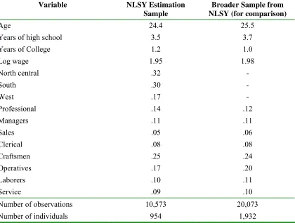
paid workers are found in the service occupation. Descriptive statistics are presented in Table 1b.

to the data. 5ppendix 5 contains further details about the data used to estimate the model, including the details of how the sample is selected, and a discussion of the representativeness of

the …nal sample.

7:; Me

as

r

t

rr

r

cc

at

s

The NLSY provides theB.S. Census occupation codes for eachJob. Interviewers question respon-dents about the occupation of each Job held during the year with the following two questions:

Khat kind of work do you doL That is, what is your occupationL Coders use these descriptions to classify each Job using the three-digit Census occupation coding scheme. Misclassi…cation of occupation codes may arise from errors made by respondents when describing their Job, or from errors made by coders when interpreting these descriptions. Evidence on the extent of

misclassi…cation is provided by Mellow and SiderN19PQR, who perform a validation study of oc-cupation codes using ococ-cupation codes found in the CPS matched with employer reports of their

employeeSs occupation. They …nd agreement rates for occupation codes of 5P% at the narrowly de…ned three digit level andP1% at the more broadly de…ned one digit level. 5dditional evidence on measurement error in occupation codes is presented by MathiowetTN1992R. MathiowetTN1992R independently creates one and three-digit occupation codes based on occupational descriptions

from employees of a large manufacturing …rm and Job descriptions found in these workerSs per-sonnel …les. The agreement rate between these independently coded one-digit occupation codes

is 76%, while the agreement rate for three-digit codes is only 52%. In addition to comparing

the three and one-digit occupation codes produced by independent coding, MathiowetT N1992R also conducts a direct comparison of the company record with the employeeSs occupational de-scription to see if the two sources could be classi…ed as same three-digit occupation. This direct

comparison results in an agreement rate of 87% at the three-digit level.

In general, papers examining occupational choices and the returns to occupation speci…c work

experience have not dealt with the di¢ cult issues raised by measurement error in occupation codes even though it is widely believed that occupation codes are quite noisy. Kork by Kambourov and Manovskii N2007R is a notable exception to this trend. They exploit the fact that the Panel Study of Income DynamicsNPSIDRoriginally coded occupations using an approach similar to the NLSY in which occupation coders translated workerSs verbatim descriptions of their occupation into an occupation code separately in each survey year. The PSID later released retrospective

occupation data …les where occupation coders were instead given access to a workerSs complete

sequence of occupational descriptions over his career. Kambourov and Manovskii X2007Y show that occupational mobility is lower in the retrospective …les, which is consistent with the

hypoth-esis that coders introduce measurement error into occupation codes when they interpret workers[ verbatim\ob descriptions. ]owever, it is important to note that while this type of retrospective coding is likely to reduce the number of false occupational transitions found in the data, it does

not provide any additional information about a worker[s true occupation. ^iven this limitation of the PSID data, Kambourov and ManovskiiX2007Y estimate the returns to occupation speci…c work experience, but they are not able to allow the wage equation to vary across occupations,

or to estimate the importance of cross occupation experience e¤ects.

_ `

cc

at

a

c

t

sc

ass

cat

xy{

A

as

sc

ass

cat

The model of occupational choices developed in this paper builds on previous models of sectoral

and occupational choices such as ]eckman and SedlacekX19

ˆ5, 1990 Y and

^ould

X2002Y. These models are all based on the framework of self selection in occupational choices introduced by‰oy

X1951Y. LetV

iqt represent the utility that workerireceives from working in occupation qat time

period t. Let N represent the number of people in the sample, let T(i) represent the number

of time periods that person i in the sample, and let Q represent the number of occupations.

Šssume that the value of working in each occupation is the following function of the wage and non-pecuniary utility,

Viqt =wiqt+Hiqt+"iqt; X1Y

wherewiqt is the log wage of person i in occupationq at timet; Hiqt is the deterministic portion

of the non-pecuniary utility that person i receives from working in occupation q at time t, and

"iqt is an error term that captures variation in the utility ‹ow from working in occupation q caused by factors that are observed by the worker but unobserved by the econometrician.

The log wage equation is

wiqt = iq+Zit q+ Q X

k=1

qkExpikt+eiqt; X2Y

where _iq is the intercept of the log wage equation for person i in occupation q, Zit is a vector

of explanatory variables, and Expikt is person i[s experience at time t in occupation k. This

speci…cation allows for a full set of cross-occupation experience e¤ects, so the parameter estimates

provide evidence on the transferability of skills across occupations. The …nal term,eiqt, represents

a random wage shock. The deterministic portion of the non-pecuniary utility Œow equation for personi is speci…ed as

Hiqt =Xit q+ Q X

k=1

qkExpikt+ Q X

k=1

qkLastoccikt+ iq; Ž

where Xit is a vector of explanatory variables and Lastocciktis a dummy variable equal to 1 if

personiworked in occupationkat timet 1. This variable allows switching occupations to have

a direct impact on non-pecuniary utility, as it would if workers incur non-pecuniary costs when

switching occupations. The …nal term, _iq; represents person is innate preference for working in occupation q. In general, sectoral choice models of this type are identi…ed even if the same

explanatory variables appear in both the wage equation and the non-pecuniary utilityŒow equa-tion. ‘owever, it is normally considered desirable to include a variable that impacts occupational choices but does not directly impact wages. In this application lagged occupational choice

dum-mies and high school and college diploma dumdum-mies are included in the non-pecuniary equation

but excluded from the wage equation. The exclusion of the lagged occupational choice dummies

from the wage equation assumes that individuals incur psychic mobility costs when switching

occupations, but there is no direct monetary switching cost. ‘owever, because occupation spe-ci…c experience e¤ects vary across occupations, when an individual switches occupations his

accumulated skills may be valued less highly in his new occupation.4

Let Oit represent the occupational choice observed in the data for person i at time t. This

variable is an integer that takes a value ranging from1toQ. “persons true occupational choice may di¤er from the one observed in the data if classi…cation error exists. Let Obit represent the

true occupational choice, which is simply the occupation that yields the highest utility,

b

Oit =q if Viqt = maxfVi1t; Vi2t; :::; ViQtg: 4

The model of misclassi…cation allows the probability of misclassi…cation to depend on the

value of the latent variable Viqt. The misclassi…cation probabilities are denoted as

jk = Pr(Oit =j j Obit=k); for j = 1; :::; Q; k= 1; :::; Q: 5 4

That is, jk represents the probability that the occupation observed in the data isj, conditional

on the actual occupational choice being k. The ™s are estimated šointly along with the other parameters in the model. The jjterms are the probabilities that occupational choices are

correctly classi…ed. There areQ Qmisclassi…cation probabilities, but there are only[(Q Q) Q]

free parameters because the misclassi…cation probabilities must sum to one for each possible

occupational choice,

Q X

j=1

jk = 1; for k = 1; :::; Q: ›œ

žollowing existing parametric models of misclassi…cation, the model assumes that the mis-classi…cation probabilities f jk : k = 1; ::; Q; j = 1; :::; Qg depend only on j and k, and not on

the other explanatory variables in the model. One possible shortcoming of this baseline model

of occupational misclassi…cation is that it rules out person speci…c heterogeneity in the

propen-sity to misclassify occupations that may be present in panel data such as the NLSY. Section

Ÿ.4 of this paper presents an extension of the model that allows for this type of within-person correlation in misclassi…cation rates.

It is necessary to specify the distributions of the error terms in the model before deriving the

likelihood function.  ssume that "iqt iid extreme value and eiqt N(0;

2

eq). Let i represent

a Q 1 vector of personi™s preferences for working in each occupation, and let

i represent the

Q 1 vector of person i™s log wage intercepts in each occupation. Let F( ; ) denote thešoint distribution of the wage intercepts and occupational preferences.

Let represent the vector of parameters in the model, =f _k; _kj; _kj; kj; k; jk; ek; F( ; ) :

k = 1; :::; Q; j = 1; :::; Qg: žor brevity of notation, when it is convenient I suppress some or all of the argumentsf ; Zit; Xit; Expikt; Lastoccikt; wobsit gat some points when writing equations for

probabilities and likelihood contributions, even though the choice probabilities and likelihood

contributions are functions of all of these variables. De…ne Pbit(q; wobsit ) as the šoint probability that personi chooses to work in occupationq in time period t and receives a wage ofwobs

it . The

outcome probability is

b

Pit( q; wobsit j ; ) = Pr(Viqt = maxfVi1t; Vi2t; :::; ViQtg jwiqt =wobsit ) Pr(wiqt =witobs): ›7

There is no closed form solution for this probability, so it is approximated using simulation

meth-ods. This involves taking random draws from the distribution of the errors, and computing the

mean of the simulated probabilities.5 _{The likelihood function for the observed data is constructed}

5

using the misclassi…cation probabilities and the true choice probabilities. De…ne Pit(q; wobsit ) as

the probability that person i is observed working in occupation q at time period t with a wage

ofwobs

it . This probability is the sum of the true occupational choice probabilities weighted by the

misclassi…cation probabilities,

Pit(q; witobs j ; ) = Q X

k=1

qkPbit(k; wobsit j ; ): £¤¥

Note that the outcome probability imposes the restriction that the observed wage is drawn

from the worker¦s actual occupation, which rules out situations where a worker intentionally misrepresents his occupation and simultaneously provides a false wage consistent with the false

occupation. The likelihood function is simply the product of the probabilities of observing the

sequence of occupational choices observed in the data for each person over the years that they

are in the sample,

L( ) =

N Y

i=1

Z T_Y(i)

t=1

Q X

q=1

1fOit =qgPit(q; witobs j ; )dF( ; ) £9¥

=

N Y

i=1

Z

Li( j ; )dF( ; ); £10¥

where 1f g denotes the indicator function which is equal to 1 if its argument is true and 0

otherwise. The likelihood function must be integrated over the §oint distribution of skills and preferences, F( ; ). ¨ollowing ©eckman and Singer £19¤4¥, this distribution is speci…ed as a discrete multinomial distribution.ª

Suppose that there areM types of people, each with a Q 1

vector of wage intercepts m_{andQ 1vector of preferences} m_{. Let}

!mrepresent the proportion

of the mth type in the population. The unconditional likelihood function is simply a weighted

form solution. « ¬ a result it is straightforward to use a smooth simulator for the probabilities in the likelihood function. During estimation, ­ ® draws from the distribution of the errors are used to simulate the integral. « ¯tithetic acceleration is used to reduce the variance of the simulated integral. « ¬a check on the sensitivity of the estimates to the number of simulation draws the° ±² ³ ´³ µ ¶²ion routine was re-started using­ ® ® draws. The parameter estimates· ¶¯¸ value of the likelihood function at the maxim¹ ´º were essentially unchanged by this increase in the number of simulation draws.

»

average of the type speci…c likelihoods,

L( ) =

N Y

i=1

Z

Li( j ; )dF( ; )

=

N Y

i=1

M X

m=1

!mLi( j i = m

; i = m

)

=

N Y

i=1

Li( ) ¿11À

ÁÂÃ ÄÅ

a

at

t

ct

The maÒor complication in evaluating the likelihood function arises from the fact that classi…ca-tion error in occupaclassi…ca-tion codes creates non-classical measurement error in the observed occupaclassi…ca-tion

speci…c work experience variables and previous occupational choice dummy variables that

de-scribe an individualÓs state. This implies that the true state of each agent is unobserved. Previous research into occupational choices has not addressed this issue. The key to understanding the

so-lution to this problem is to realiÔe that the model of misclassi…cation implies a distribution of true values of occupation speci…c work experience and lagged occupational choices for each individual

in each time period. Estimating the parameters of the model by maximum likelihood involves

integrating over the distribution of these unobserved state variables. Õowever, there is no closed form solution for this integral, and, more importantly, the distribution is intractably complex.

These problems are solved by simulating the likelihood function. The algorithm involves

recur-sively simulating R sequences of occupation speci…c work experience and lagged occupational

choices that span a workerÓs entire career. The individualÓs likelihood contribution is computed for each simulated sequence, and the path probabilities are averaged over the R sequences to

obtain the simulated likelihood contribution. Ö detailed description of the simulation algorithm is presented in Öppendix B.

ÁÂ Á

×ÐÌÉ

t

cat

This section presents the identi…cation conditions for the occupational choice model with

mis-classi…cation and discusses several related issues.

ÙÚÙÚÛ ÜÝÞßtàácatàâß ãâßÝàtàâ ßs

The identi…cation conditions for a model of misclassi…cation in a binary dependant variable are

presented by äausman, åbrevaya, and Scott-Morton æ199çè. This condition is extended to the case of discrete choice models with more than two outcomes byéamalhoæ2002è. The parameters of the model are identi…ed if the sum of the conditional misclassi…cation probabilities for each

observed outcome is smaller than the conditional probability of correct classi…cation. In the

context of the occupational choice model presented in this paper this condition amounts to the

following restriction on the misclassi…cation probabilities,

X

k6=j

jk < jj; j = 1; :::; Q: æ12è

This condition implies that it is not possible to estimate the extent of misclassi…cation along

with the rest of the parameter vector if the quality of the data is so poor that one is more likely

to observe a misclassi…ed occupational choice than a correctly classi…ed occupational choice.

ÙÚÙÚê ëàscìssàâß

Estimating the extent of classi…cation error in the NLSY occupation data along with the

parame-ters of the occupational choice model is only possible if one is willing to adopt a parametric model

along with the associated functional form and distributional assumptions.7 _{It is worthwhile to}

consider at an intuitive level how the parametric occupational choice model and misclassi…cation

model are linked together. Let e represent the parameter vector for the occupational choice model, and let _e represent the vector of misclassi…cation parameters. íiven e, the parametric model of occupational choices provides the probability that each occupational choice and wage

combination observed in the NLSY is generated by the model. Taking e as given, one could choose the value of _e that maximiîes the probability of observing the NLSY occupation and wage data. Broadly speaking, this will happen when the combinations of occupational choices

and wages that are unlikely to be generated by the model at the parameter vector eare assigned a relatively high probability of being a¤ected by misclassi…cation. During estimation, e is not …xed, it is estimated simultaneously with _e, so estimating the model amounts to choosing the value of ethat best …ts the data, with the added consideration that the chosen value of _e allows misclassi…cation to account for some of the observed patterns in the data.

7_{It should be noted that as is the case with all parametric models of this type, if the model is mis-speci…ed,} parameter estimates will be biased.

Existing parametric models of misclassi…cation estimate misclassi…cation rates using discrete

choice models, while in contrast this paper ïointly models discrete occupational choices along with wages. The advantage of this approach is that to the extent that wages vary across

occupa-tions, observed wages provide information about which observed choices are likely to be a¤ected

by misclassi…cation.ð

This approach uses information about the relationship between observable

variables ñsuch as educationò and occupational choices, along with information about the con-sistency of observed wages with reported occupations to infer the extent of misclassi…cation in

the data. It should be noted that when occupations are measured with error, it is not possible

to nonparametrically determine the exact relationship between true occupational choices, wages,

and observable variables such as education. óowever, within a particular parametric model of occupational choices and wages, these parameters can be estimated. 9

The availability of validation data on occupations from an outside data source would, in

principle, allow one to relax some of the parametric assumptions adopted in this paper. ôor example, if another data set contained information about reported occupations, true occupations,

and possibly other explanatory variables, this information could be used to integrate out the e¤ect

of measurement error. Of course, this approach relies on the assumption that the measurement

error process is identical in the two sources of data. õhile this approach appears promising and is certainly worth pursuing in future research, on a practical level adopting this approach

would most likely require additional data collection that was targeted speci…cally at validating

occupation codes.10 _{One possible approach would be to validate an individual}

ös occupation by ÷

In the extreme case where the wage distribution is identical across occupations observed wages do not pro-vide any additional information about misclassi…cation. øowever, even if the unconditional wage distribution is identical across occupations, if the wage distribution in each occupation is a function of observable characteristics

ùú ûch as education and occupation speci…c experienüýþ ÿ and the e¤ects of these variables on wages vary across occupations, then observed wages will still provide information about misclassi…cation.

9

Ahough panel data is used to estimate the model, it is also possible to estimate this type of model using cross sectional data. Aúan experiment, I randomly selected a cross section of workers from the panel data NLSY sample and re-estimated the model. The estimated level of misclassi…cation in the cross sectional version of the model was 8ÿ compared to 9% in the panel data version. The fact that these estimates are so close suggests that misclassi…cation rates are primarily identi…ed by the consistency of an indiv ûs reported occupation with the cross sectional distribution of choices, wages, and observable variables, rather than by the extent to which an observed occupational choice is consistent with an individual workers observed sequence of career choices.

10_{The ma}

jor problem is that existing validation studies, such as the 1977 supplement to the CPS, question respondents about their occupation and then attempt to validate the reported occupations by surveying employers. In general there is no reason to be con…dent that the employer surveys provide occupation data that is free from error. Depending on the information contained in personnel …les and the system that an employer uses to categorize employees, the responses provided by …rms could in fact be noisier than those provided by individuals. Aú a result, it is generally accepted that these validation studies provide an upper bound on the extent of measurement error. In contrast, validating wage data appears to be a much simpler task, since one would expect that …rms could normally provide accurate salary information from their payroll records.

questioning his supervisor, since presumably supervisors know the type of work performed by

workers that they manage. This approach would circumvent some of the problems associated

with validating occupation codes using personnel records, which may or may not contain ob descriptions that accurately re‡ect occupations.

3.4

A

t

t

r

t

sc

ass

cat

at

s

The model of misclassi…cation presented in Section .1 assumes that all individuals have the same probability of having one of their occupational choices misclassi…ed. In a panel data

setting such as the NLSY, it is possible that during the yearly NLSY interviews some individuals

consistently provide poor descriptions of their obs that are likely to lead to measurement error in the occupation codes created by the NLSY coders. On the other hand, some workers may

be more likely to provide accurate descriptions of their occupations that are extremely unlikely

to be misclassi…ed. The remainder of this section extends the occupational choice model with

misclassi…cation to allow for time persistent misclassi…cation by using an approach similar to the

one adopted by Dustmann and van Soest (2001) in their study of misclassi…cation of language

‡uency.

The primary goal of the extended model is to allow for person-speci…c heterogeneity in

mis-classi…cation rates in a way that results in a tractable empirical model. Suppose that there

are three subpopulations of workers in the economy, and that these subpopulations each have

di¤erent probabilities of having their occupational choices misclassi…ed. De…ne the occupational

choice misclassi…cation probabilities for subpopulationy as

jk(y) = Pr(Oit=jjObit=k); j = 1; :::; Q; k = 1; :::; Q; (1)

Q X

j=1

jk(y) = 1; k= 1; :::; Q; y= 1;2;3: (14)

Denote the proportion of subpopulationyin the economy as (y);wherey= 1;2;3and

3

X

y=1

(y) =

1:This speci…cation of the misclassi…cation rates allows for time-persistence in misclassi…cation,

since the jk(y)’s are …xed over time for each subpopulation. During estimation the (y)’s and

jk(y)’s of each subpopulation are estimated along with the other parameters of the model, so it is necessary to specify the misclassi…cation model in such a way that the number of parameters

in the model does not become unreasonably large. In order to keep the number of parameters

at a tractable level, the number of subpopulations is set to a small number , and the

mis-classi…cation probabilities are restricted during estimation so that the occupational choices of

subpopulation 1 are always correctly classi…ed.11

This model of misclassi…cation incorporates the key features of heterogeneous

misclassi…ca-tion rates in a fairly parsimonious way. Some fracmisclassi…ca-tion of the populamisclassi…ca-tion (1)is always correctly classi…ed, and the remaining two subpopulations are allowed to have completely di¤erent

mis-classi…cation rates, so that both the overall level of mismis-classi…cation and the particular patterns

in misclassi…cation are allowed to vary between subpopulations.

The likelihood function presented in section.1 can be modi…ed to account for person-speci…c heterogeneity in misclassi…cation. The observed choice probabilities are easily modi…ed so that

they are allowed to vary by subpopulation,

Pit(q; witobs j ; ; y) = Q X

k=1

qk(y)Pbit(k; wobsit j ; ); 15

wherey= 1;2;3indexes subpopulations. Conditional on subpopulations, the likelihood function

is

L( jy) =

N Y

i=1

Z T_Y(i)

t=1

Q X

q=1

1fOit=qgPit(q; witobs j ; ; y)dF( ; ) 16

=

N Y

i=1

Z

Li( j ; ; y)dF( ; ); 17

The subpopulation that a particular person belongs to is not observed, so the likelihood function

must be integrated over the discrete distribution of the type-speci…c misclassi…cation rates,

L( ) =

N Y

i=1 3

X

y=1

M X

m=1

(y)!mLi( jy; i = m_;

i =

m_{) 1}

=

N Y

i=1

Li( ):

P

ara

t

r

st

at

s

This section presents the simulated maximum likelihood parameter estimates for the occupational

choice model. First, the parameters that reveal the extent of classi…cation error in reported occu-pations are discussed, and then the parameter estimates from the occupational choice model that

11_{This version of the model already has 421 parameters that must be estimated, so in order to keep the model} tractable it was never estimated with more than three subpopulations.

corrects for classi…cation error and allows for person-speci…c heterogeneity in misclassi…cation

are compared to the estimates from a model that does not correct for measurement error. Next,

the sensitivity of the estimates to measurement error in wages is examined. inally, the model is used to simulate data that is free from classi…cation error in occupation codes.

1 Th

t

t

as

r

t

rr

r

cc

at

s

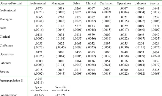
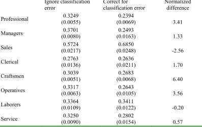
The estimates of the misclassi…cation probabilities for subpopulations 2 and along with the estimated proportions of each type in the population are presented in Panels and B of Table

. The bottom row of panel shows that correcting for classi…cation error results in a large improvement in the …t of the model, since the likelihood function improves from 18;695 when

classi…cation error is ignored to 17;821 when classi…cation error is corrected for. The

proba-bility in row i, column j is the estimate of ij(y), which is the probability that occupation i is

observed in the data conditional on occupation j being the actual choice for a person in

subpop-ulationy. or example, the entry in the third column of the …rst row indicates that condition of being a member of subpopulation 2, there is a2:6% chance that a person who is actually a sales

worker will be misclassi…ed as a professional worker. The diagonal elements of the two panels

of Table show the probabilities that occupational choices are correctly classi…ed. veraged across all occupations, the probability that an occupational choice is correctly classi…ed is .868

for subpopulation 2 and:840 for subpopulation. One striking feature of the estimated misclas-si…cation probabilities is that they provide substantial evidence that misclasmisclas-si…cation rates vary

widely across occupations. or example, in subpopulation 2 the probability that an occupational choice is correctly classi…ed ranges from a low of :56for sales workers to a high of :99for

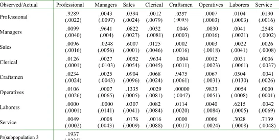
crafts-men, while in subpopulation the probability that an occupational choice is correctly classi…ed ranges from a low of:60 for sales workers to a high of :98for operatives.

The estimates of the probabilities that a person belongs to subpopulations 2 and are42% and 19%, which leaves an estimated 38% of the population belonging to subpopulation 1, the

group whose occupational choices are never misclassi…ed. The fact that a substantial fraction of

the population belongs to the subpopulation whose occupational choices are never misclassi…ed

highlights the importance of allowing for person-speci…c heterogeneity in misclassi…cation rates.

When averaged over subpopulations, the subpopulation-speci…c misclassi…cation rates indicate that 91% of one-digit occupational choices are correctly classi…ed. This estimate of the overall

extent of misclassi…cation in the NLSY data is lower than the misclassi…cation rates reported in

validation studies based on other datasets. or example, Mellow and Sider 19!"# …nd an agree-ment rate of81% at the one-digit level between employee$s reported occupations and employer$s occupational descriptions in the January 1977 Current Population Survey CPS#. Mathiowet% 1992# …nds a 76% agreement rate between the occupational descriptions given by workers of a single large manufacturing …rm and personnel records.12

One possible explanation for the lower misclassi…cation rate found in this study compared to

the validation studies is that the NLSY occupation data is of higher quality than both the CPS

data and the survey conducted by Mathiowet% 1992#. It appears that the procedures used by the CPS and NLSY in constructing occupation codes are quite similar, so it is not clear that one

should expect the NLSY data to have a lower misclassi…cation rate than the CPS.&n alternative explanation is that the employer reports of occupation codes that are assumed to be completely

free from classi…cation error in validation studies are in fact measured with error.1'

If this is true,

then comparing noisy self reported data to noisy employer reported data would cause validation

studies to overstate the extent of classi…cation error in occupation codes. The idea that this

type of validation study may result in an overstatement of classi…cation error in occupation or

industry codes is not a new one. or example, Krueger and Summers 19!!# assume that the error rate for one-digit industry classi…cations is half as large as the one reported by Mellow

and Sider 19!"# as a rough correction for the overstatement of classi…cation error in validation studies.

The wide variation in misclassi…cation rates across occupations along with the patterns in

misclassi…cation suggest that certain types of *obs are likely to be misclassi…ed in particular directions. In addition, the misclassi…cation matrix is highly asymmetric. or example, there is only a 1.4% chance that a manager will be misclassi…ed as a sales worker, but there is a 21%

chance that a sales worker will be misclassi…ed as a manager. +eading down the laborers column of panel & of Table " shows that laborers are frequently misclassi…ed as service workers 22%#, but service workers are very unlikely to be misclassi…ed as laborers ."9%#. urther evidence of asymmetric misclassi…cation is found throughout Table ".

12_{This study is the …rst to estimate a parametric model of occupational misclassi…cation, so the validation} studies provide the only basis for comparison for the estimated misclassi…cation rates.

1,

It is widely acknowledged that although validation studies are frequently based on the premise that one source of data is completely free from error, in reality no source of data will be completely free from measurement error. See Bound, Brown, and Mathiow-/ 025 7 7 9 ;for a discussion of this issue.

<=> ?

cc

at

a

c

ara

t

r

st

at

s

The parameter estimates for the occupational choice model estimated with and without correcting

for classi…cation error are presented in Table 4. In addition, this table presents a measure of

the di¤erence between each parameter in the baselineY

bZ and classi…cation error Y

ceZmodels,

( b ce)=se( ce); where se( ce) is the standard error of ce. In the remainder of the paper

this standard error normali[ed di¤erence will be referred to as the normali[ed change in the parameter.

\]^]_ `aab cqkatrst

while theoretical results regarding the e¤ects of measurement error in simple linear models have been derived, there are no clear predictions for nonlinear models such as this occupational choice

model. Broadly speaking, one would expect the patterns of misclassi…cation present in the data

to be a key determinant of the magnitude and direction of the resulting bias. Due to the large

number of wage equation parameters, this discussion focuses on a small subset of parameter

estimates with the goal of demonstrating that classi…cation error is something that needs to be

accounted for when estimating occupation speci…c wage equations. In addition, this discussion

will attempt to highlight the type of questions in general that one might receive misleading

answers to if one examines occupational choices and ignores misclassi…cation.

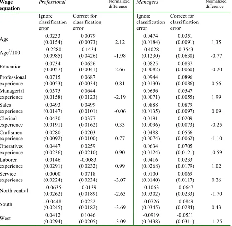
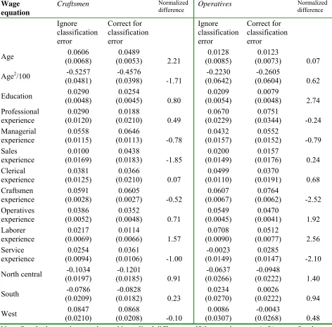
The wage equation parameter estimates are presented in Panel { of Table 4. The estimates of the wage equation for the professional occupation show a number of large changes in the

es-timated e¤ects of occupation speci…c work experience on wages between the model that ignores

classi…cation error in occupations and the one that accounts for classi…cation error. |or ex-ample, the e¤ect of a year of managerial experience on wages in the professional occupation

is biased downward by 42% from :064 to :037 when misclassi…cation is ignored. The standard

error normali[ed di¤erence for this parameter is -2.19, so the bias appears relatively large rel-ative to the standard error. The bias in this particular parameter is also interesting because

the estimated misclassi…cation probabilities show that professionals are rarely misclassi…ed as

managers Y 21(2) =:0066; 21(3) =:0099Z, and managers are rarely misclassi…ed as profession-als Y 12(2) = :0018; 12(3) = :0043Z. The low misclassi…cation rates between these occupations combined with the large bias in the experience coe¢ cient illustrates the point that even a small amount of misclassi…cation can produce large biases in estimates of the transferability of human

capital across occupations.

Sales workers are the most frequently misclassi…ed workers in both subpopulations 2 and ~.

veraged across all three subpopulations, only 72% of sales workers are correctly classi…ed. In the most common subpopulation, sales workers are most likely to be misclassi…ed as managers

€ 23(2) =:21, so one might expect signi…cant bias in estimates of the parameters of the man-agerial and sales wage equations. The estimates show that ignoring classi…cation error causes

the value of experience as a manager in the managerial occupation to be overstated by 19%

€normali‚ed change ƒ 1.99. In addition, ignoring classi…cation error leads to the misleading conclusion that one year of clerical experience increases wages by nearly 1~% in the sales occupa-tion, and this e¤ect is statistically signi…cant at the 5% level. „owever, once classi…cation error is corrected for, the estimated e¤ect of clerical experience on sales wages falls by 2†~, and the e¤ect is not statistically di¤erent at conventional levels. Similarly, ignoring classi…cation error

leads to an overstatement in the value of professional experience in the sales occupation €.0ˆ72 vs. .0~0‰, although the normali‚ed di¤erence for this parameter is only .ˆ7.

Šurther evidence of large changes in estimates of the transferability of human capital across occupations is found in the craftsman occupation. The model that does not correct for

classi…-cation error implies that a year of professional experience increases a craftsman‹s wages by2:9%, and this e¤ect is statistically signi…cant at the 5% level: Once classi…cation error is accounted

for this e¤ect falls to 1:8% and it is not statistically di¤erent from ‚ero at the 5% level. This …nding suggests that the type of skills accumulated during employment as a professional have

little or no value in craftsmanŒobs. It appears that the false transitions created by classi…cation error lead to an overstatement of the transferability of human capital between the professional

occupation and this seemingly unrelated lower skill occupation.

nother way of comparing the wage equations in the baseline and measurement error model is to determine the number of hypothesis tests where the results of the test change between

the baseline and classi…cation error models. Šor example, one hypothesis that is commonly of interest is the null hypothesis that the e¤ect of each individual explanatory variable on wages

equals ‚ero. Comparing the results of these hypothesis tests for the baseline model and the classi…cation error model shows that the reŒection or acceptance of the null hypothesis at the 5% level changes for17 variables in the wage equation between the two models. In other words,

ignoring classi…cation error would cause one to mistakenly accept or reŒect the null hypothesis that the e¤ect of an explanatory variable equals‚ero for 17 wage equation variables.

The …nal parameters of the wage equation are the standard deviations of the random shock

to wages in each occupation, eq, for q = 1; :::;8. The estimates of these standard deviations

show that randomuctuations in wages are overstated in six out of the eight occupations in the model that ignores classi…cation error. The intuition behind the direction of this bias is that the

model must provide an explanation for the large number of short duration occupation switches

that occur in the data. Žhen classi…cation error is ignored, the model accomplishes this through relatively large transitory wage shocks.

The determinants of occupational choices have been the subect of considerable research interest, and several recent papers have examined the related question of the role of occupation

speci…c human capital in determining wages. lthough labor economists have typically focused on determining the roles of …rm tenure and general work experience in determining wages, new

evidence suggests that in fact occupation speci…c skills play an important role in determining

wages.14 _{Comparing the estimates of the wage equation found in this paper to existing estimates}

is di‘ cult for a number of reasons. “irst, there is no existing paper that estimates directly comparable occupation speci…c wage equations at the one-digit level. Second, existing papers

that estimate wage equations that are similar in some respects do not allow for the type of

cross-occupation experience e¤ects found in this study.15

”owever, overall the wage equation estimates appear to be broadly consistent with existing research in this area. “or example, Both Kambourov and Manovskii •2007– and Sullivan •2007– …nd that while experience in a workers—current occupation has as an important e¤ect on wages, wages are strongly impacted by total work experience. This …nding is consistent with the relatively large cross occupation

experience e¤ects reported in this paper. Keane and Žolpin •1997– also …nd relatively large cross occupation experience e¤ects between blue collar and white collar employment, which is

again broadly consistent with the wage equation estimates reported in this paper. It is also

possible to get a rough sense of how the magnitudes of the estimated e¤ects of occupation

speci…c work experience on wages in this paper compare to existing research. The estimates in

this paper suggest that when classi…cation error is ignored, averaged across all occupations one

year of occupation speci…c work experience increases wages by approximately 7%. Kambourov

and Manovskii •2007– do not report a parameter estimate that is directly comparable to this number, but combining the di¤erent parameter estimates that they report suggest that wages

14_{See, for example, Kambourov and Manovskii}

˜ ™ š š› œ and Sullivan˜™ š š›œ  15_{Kambourov and Manovskii}

˜ ™ š š›œand Sullivan˜™ š š› œconsider the special case of the wage equation estimated in this paper where all of the cross occupation experience e¤ects are equal. žowever, these studies also consider …rm tenure and industry speci…c work experience. Keane andŸolpin˜   ¡¡ › œallow for cross occupation experience e¤ects, but their work uses occupation codes aggregated to the level of blue and white collar£obs.

grow by approximately 5%-¥% with each year that a worker spends in an occupation.

¦§¨§¨ ©ª«¬­®c¯«°ar± ²t°³°t± ´³ªµs ¶ ²«ªbs®r·®¸ ¹®t®rªº®«®°t±

The occupational choice model presented in this paper allows occupational choices to depend

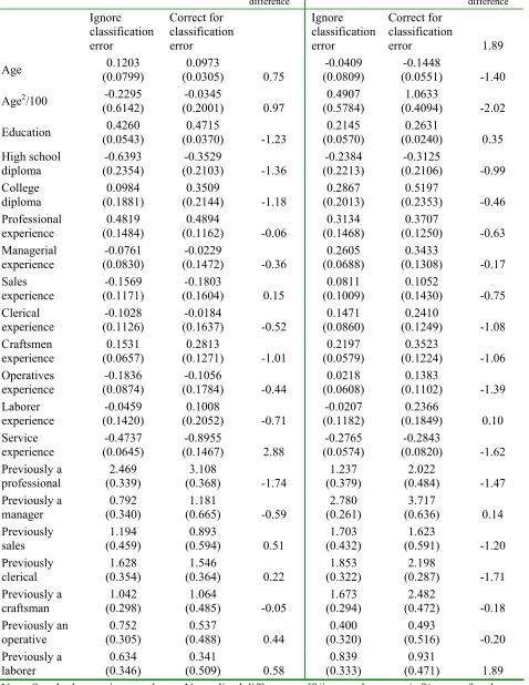
on non-pecuniary utility »ows as well as wages. The importance of modelling occupational choices in a utility maximi¼ing framework rather than in an income maximi¼ing framework is demonstrated in work by Keane and½olpin ¾1997¿and Àould ¾2002¿. The parameter estimates for the non-pecuniary utility»ow equations for the models estimated with and without accounting for classi…cation error are presented in Panel B of Table 4. These results show that ignoring

classi…cation error leads to signi…cant biases in estimates of the e¤ects of variables such as age,

education, and work experience on occupational choices.

The non-pecuniary utility »ow parameters are all measured in log-wage units relative to the base choice of service employment. Áor example, the estimate of the e¤ect of working as a pro-fessional in the previous time period on the propro-fessional utility »ow is 2:469 in the model that ignores classi…cation error. This means that a person who previously worked as a professional

re-ceives utility that is2:469log wage units higher than a person who was previously employed as a

service worker but is currently employed as a professional. The e¤ect of previous professional

em-ployment on the professional utility»ow is biased downwards by21%when classi…cation error is ignored¾normali¼ed di¤erenceÂ-1.74¿. It appears that the false transitions between occupations created by classi…cation error lead to an understatement of the importance of state dependence

in professional employment. Overall, the estimates of the e¤ects of lagged occupational choices

on current occupation speci…c utility»ows are fairly sensitive to classi…cation error.

Ãs is the case with the wage equation, another way of examining the consequences of not correcting for misclassi…cation is to determine the number of hypothesis tests where the results of

the test at the 5% level change between the baseline and classi…cation error models. Comparing

the results of these hypothesis tests for the baseline model and the classi…cation error model show

that the reÄection or acceptance of the null hypothesis that the e¤ect of each variable equals¼ero changes for 22variables in the non-pecuniary utility »ow equation between the two models. In other words, ignoring classi…cation error would cause one to mistakenly accept or reÄect the null hypothesis that the e¤ect of an explanatory variable on non-pecuniary utility equals ¼ero for 22 variables.

The estimates of the wage intercepts ¾ Ås¿ and non-pecuniary intercepts ¾ Ås¿ for the three

types of people in the model are presented in Panel C of Table 4. These parameter estimates

reveal the extent of unobserved heterogeneity in skills and preferences for employment in each

occupation. The …nal section of Panel C of Table 4 shows the averages of the wage and

non-pecuniary intercepts across the three types of people for the models that correct for and ignore

classi…cation error in occupation codes. The largest bias among these parameters occurs in

parameters that measure preferences for employment in each occupation Æ ÇsÈ. Éor example, the average preference for working as a craftsman changes from :048 in the model that ignores

classi…cation error to :23 in the model that corrects for classi…cation error. Biases of similar

magnitudes are found in the average preferences for employment as operatives and laborers. The

relatively large biases in estimates of preference parameters caused by ignoring classi…cation error

occurs because unobserved heterogeneity in preferences helps explain occupational transitions

that are not well explained by the other parts of the model. Êhen classi…cation error is ignored and all occupational transitions are treated as true occupation switches, the model attempts to

explain transitions that are not well explained by wages or the deterministic portion of

non-pecuniary utility Ëows in part through preference heterogeneity.

Ì ÍÎÏÐÑ

at

ata t

at

s

r

r

sc

ass

cat

One application of the model presented in this paper is that the estimated model can be used

to simulate occupational choice data that is free from classi…cation error. The simulated data is

used to examine which workers tend to be identi…ed as misclassi…ed by the model, the predicted

patterns in misclassi…cation over workersÇcareers, and the predicted relationship between wages and misclassi…cation.

ÜÝÞ ßàáâã

at

cc

at

a

c

s

ìíîíî ïðñcð ïòróôrs arô õñscöassñ÷ôøù

One explanatory variable that is of central importance when investigating occupational choices

is education, since there is strong sorting across occupations based on completed education.

úiven this fact, it is useful to see how completed education levels vary between choices that are identi…ed as misclassi…ed choices in the simulated data compared to choices that are identi…ed

as correctly classi…ed choices.

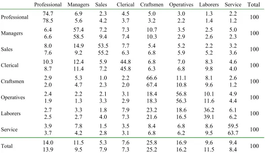
Table 5 shows the distribution of completed education for correctly classi…ed and misclassi…ed

occupational choices, disaggregated by occupation. ûor example, the table shows that the model predicts that 10.ü% of those workers who are correctly classi…ed as professionals have not com-pleted any years of college, while 4ü.ý% of workers who are misclassi…ed as professionals have not completed any years of college. þ correctly classi…ed professional has a 71.ü% change of being a college graduate, while a worker misclassi…ed as a professional has only aÿ0.2% chance of being a college graduate. Clearly, education serves as a strong predictor of which observations are likely

to be true professionals as opposed to observations that are falsely classi…ed as professionals.

These results are consistent with the fact that thejobs located in the professional occupation are overwhelmingly ones that require a college degree, or at least some amount of completed higher

education.

þcross the other occupations, similarly strong and sensible relationships exist between ed-ucation and misclassi…cation. ûor example, in blue collar occupations, one would expect to see the opposite relationship between misclassi…cation and education from the one found in the

professional occupations. This is in fact what the results in Table 5 show. ûor example, the percentage of correctly classi…ed workers who have graduated from college is 2.1% for craftsmen,

2.5% for operatives, andÿ.2% for laborers. In contrast, for workers who are falsely classi…ed in these occupations the percentage of workers who are college graduates is 1ü.7% for craftsmen, 21.5% for operatives, and 11.7% for laborers. In general, the model tends to‡ag workers as mis-classi…ed who have reported education levels that appear to be inconsistent with their reported

occupation.

5.1.2 The Frequency of Misclassi…cati on Over an Indivi dual’s Career

Given the panel nature of the data, the simulated occupational choice data can be used to examine how often occupational choices are misclassi…ed over a typical individual s career. Table

ýpresents the distribution of the total number of times that occupational choices are misclassi…ed over the course of a person s career. The majority of workers never experience misclassi…cation

(57.2%), 17.ý% of workers are misclassi…ed once over their career, and very few workers are misclassi…ed more than …ve times over their career (4.ÿ%). Table ý also provides information about the distribution of the lengths of misclassi…cation spells. ûor example, the …rst entry in the …nal column of Tableýshows that conditional on an occupational choice being misclassi…ed, there is a 72.9% chance that the person will be correctly classi…ed in the next survey. Conditional on

being misclassi…ed, there is an 18.3% chance that a person will be misclassi…ed in two consecutive periods, and there is only a 5.2% chance that a person will be misclassi…ed in three consecutive

periods.16

r ccpat a cs, bsr cs, a Wags

Table 7 shows the average true occupational choice probabilities conditional on observed choices

and observed wages that are predicted by the empirical model. This analysis shows how the

classi…cation error rates generated by the model vary with observed wages and provides a more

detailed analysis of the type of occupational choice and wage combinations that are likely to be

a¤ected by classi…cation error.

Observed occupational choices are listed in the far left column of Table 7, while actual

oc-cupational choices are listed in the top row. Conditional on the observed choice and wage and all of the other explanatory variables, the model is used to calculate the conditional probability that the actual choice is each of the eight occupations for each occupational choice observed in

the data. The average of each probability for each occupation is presented in Table 7.

Proba-bilities are disaggregated by the percentile of the observed wage in the wage distribution of the

observed occupation to show how misclassi…cation rates vary with observed wages. or example, the top left cell of Table 7 shows that a worker observed in the data as a professional worker

with a wage in the top 10% of the professional wage distribution has a 90.9% chance of being

correctly classi…ed as a professional worker. However, a worker observed as a professional with a wage in the bottom 10% of the professional distribution has only a 75.7% chance of actually

being a professional worker. People observed in the data as low wage professional workers are

primarily service workers 9.5%.

Similar patterns of misclassi…cation are found in the sales and clerical occupations, where

workers in certain areas of the wage distribution are more likely to be misclassi…ed than those in

other areas of the wage distribution. or example,91:6%of clerical workers in the top10%of the clerical wage distribution are correctly classi…ed, but3:9%of those observed as high wage clerical

workers are actually professionals. However, the unconditional probability that a professional is misclassi…ed as a clerical worker is much lower 41(2) =:013; 41(3) =:013.

1

One implication of the relatively short durations of misclassi…cation spells is that the model does not tend to repeatedlyag individuals as misclassi…ed who have consistently highor lowwages for their reported occupation over the course of their entire career.

S

s

t

t

A

a

s

s

as

r

t

rr

r

a

s

One important question regarding the model presented in this paper is the sensitivity of the

results to the existence of measurement error in wages. One way of addressing this question is

to simulate noisy wage data, re-estimate the model using the noisy wage data &leaving the rest of the NLSY data unchanged', and see how the estimates of misclassi…cation parameters change when the noisy wage data is used in place of the actual wages found in the NLSY data. The

noisy wages (wme

it )are generated using the following equation,

wmeit =w obs

it + it; where it N(0; 2): &19'

Recall thatw

obs

it is a log wage, so the extent of measurement error in the noisy log wage data

is captured by 2_.

A number of validation studies have quanti…ed the extent of measurement error in wages, see Bound, Brown, and Mathiowetz&2001'for a thorough survey of this literature.

Actual estimates of

2 _{do not exist for the NLSY, so in simulating the noisy data the measurement}

error term is set towards the upper end of the reported estimates found in the literature based

on other data sources. The exact value used is 2 _{=:10:This value of} 2 _{creates a substantial}

amount of measurement error in the noisy wage data, since in the noisy data, measurement error

accounts for approximately one third of the total variation in log wages.

Rather that presenting a complete set of parameter estimates for the misclassi…cation model estimated using the noisy data, it is su¢ cient to summarize the overall e¤ect that the noisy wage data has on the parameter estimates. *hen the noisy wage data is used in place of the NLSY wage data the average parameter in the model changes by approximately 2%, so it

appears that the overall bias introduced by measurement error is relatively small. The primary

concern about measurement error in wages is that it may impact the estimates of the extent of

measurement error in occupation codes. The overall extent of misclassi…cation is summarized by the diagonal elements of the misclassi…cation rate matrices for subpopulations two and three,

jj(y); j = 1; :::; Q; y = 2;3. Across both subpopulations, the use of noisy wage data results in the average probability of correct classi…cation decreasing by only :006 from :8546 to :8486.

Adding measurement error slightly increases the overall estimated rate of misclassi…cation, but the magnitude of the increase is quite small. The corresponding average absolute change in

the probability of correct classi…cation is only :008, and the average change in the o¤-diagonal

elements is only :0015, so it appears that estimates of the overall extent of misclassi…cation in

the NLSY occupation data are quite robust to measurement error in wages.

There are a number of reasons why the estimates of the misclassi…cation parameters are

robust to a relatively large amount of measurement error in wages. The …rst reason is that,

as discussed earlier in the paper, wages are not the only source of information that the model

uses to infer that an occupational choice is misclassi…ed. -nother key point is that many of the occupational choices that are /agged in the simulations as misclassi…cations are associated with extremely large di¤erences between the reported wage and the average wage in the reported

occupation. Di¤erences of this magnitude are unlikely to be generated in large numbers by a

reasonable amount of measurement error in wages. 0or example, the median wage for workers who are identi…ed in the simulations as falsely classi…ed professionals is45.59, while the median wage for workers who are correctly classi…ed as professionals is 410.72.

9 ;<=

c

s

-lthough occupational choices have been a topic of considerable research interest, existing re-search has not studied occupational choices in a framework that addresses the biases created by

classi…cation error in self-reported occupation data. This paper develops an approach to

estimat-ing a panel data occupational choice model that corrects for classi…cation error in occupations

by incorporating a model of misclassi…cation within an occupational choice model. Estimating

this model provides a solution to the problems created by measurement error in the discrete

de-pendant variable of an occupational choice model. Methodologically, this approach contributes

to the literature on misclassi…cation in discrete dependant variables by demonstrating how

sim-ulation methods can be used to address the problems created in a panel data setting where

measurement error in a discrete dependant variable creates measurement error in explanatory

variables. The simulation technique is applicable to any discrete choice panel data model where

misclassi…cation in a current period dependent variable creates measurement error in future

ex-planatory variables. This paper also contributes to the literature on misclassi…cation by using

observed wages within the framework of an occupational choice model to obtain information

about misclassi…ed occupational choices.

The main …ndings of this paper are that a substantial number of occupational choices in the

NLSY are a¤ected by misclassi…cation, with an overall misclassi…cation rate of 9%. The results

also suggest that person-speci…c heterogeneity in misclassi…cation rates is an important feature

of the data. -n estimated7B% of the population never experiences a misclassi…ed occupational choice, and the remaining two subpopulations have substantially di¤erent propensities to have

their occupational choices misclassi…ed in particular directions. The parameter estimates also

indicate that misclassi…cation rates vary widely across occupations, and that the probability of

a worker being misclassi…ed into each occupation is strongly inDuenced by the workerJs actual occupation. Most importantly, this paper demonstrates the large bias in parameter estimates

that results from estimating a model of occupational choices that ignores the fact that

occupa-tions are frequently misclassi…ed. Consistent with existing research in the area of misclassi…ed

dependant variables, the results show that even relatively small amounts of misclassi…cation

cre-ates substantial bias in parameter estimcre-ates. Especially large biases are found in parameters

that measure the transferability of occupation speci…c work experience across occupations, since

these parameters are quite sensitive to the false occupational transitions created by classi…cation

error.

Overall, the results indicate that one should use caution when interpreting the parameter

estimates from occupational choice models that are estimated without correcting for classi…cation

error in self-reported occupations. In addition, these results suggest that similar bias may arise

when occupation dummy variables are used as explanatory variables, as is commonly done in a

wide range of studies. K possible avenue for future research would be to investigate the e¤ects of classi…cation error in occupation codes on parameter estimates in this wider class of models,

such as simple wage regressions that make use of self-reported occupation data.

Table 1a: Description of Occupations

One-Digit Occupation Mean Wage Example Three-Digit Occupations Professional, technical & kindred

workers $11.19

Accountants, chemical engineers, physicians, social scientists

Managers & administrators $12.89 Bank officers, office managers, school administrators

Sales workers $9.05 Advertising salesmen, real estate agents, stock and bond salesmen, salesmen and sales clerks Clerical & unskilled workers $7.48 Bank tellers, cashiers, receptionists, secretaries

Craftsmen & kindred workers $8.53 Carpenters, electricians, machinists, stonemasons, mechanics

Operatives $7.20 Dry wall installers, butchers, drill press operatives, truck drivers

Laborers $7.01 Garbage collectors, groundskeepers, freight handlers, vehicle washers

Service workers $6.34 Janitors, child care workers, waiters, guards and watchmen

Notes: Based on the U.S Census occupation codes found in the 1979 cohort of the NLSY. Wages are in 1979 dollars.

Table 1b: Descriptive Statistics

Variable NLSY Estimation

Sample

Broader Sample from NLSY (for comparison)

Age 24.4 25.5

Years of high school 3.5 3.7

Years of College 1.2 1.0

Log wage 1.95 1.98

North central .32 -

South .30 -

West .17 -

Professional .14 .12

Managers .11 .11

Sales .05 .06

Clerical .08 .08

Craftsmen .25 .24

Operatives .17 .20

Laborers .10 .11

Service .09 .10

Number of observations 10,573 20,073 Number of individuals 954 1,932