Algorithm for a PSO Tuned Fuzzy Controller of a DC Motor

Algorithm for a PSO Tuned Fuzzy Controller of a DC

Motor

Debasmit Das

Department of Electrical Engg. Indian Institute of Technology,

Roorkee, India

Arka Ghosh

Department of Electrical Engg. Indian Institute of Technology,

Roorkee, India

ABSTRACT

Determination of the parameters of the membership functions of a fuzzy logic control process is the crucial factor for providing optimum performance of the system. These parameters are regarded as variables and are tuned through Particle Swarm Optimization (PSO). The shape of the membership functions vary according to the variables. Consequently, the fuzzy control output changes and so does the performance. The results give an insight to the efficiency of PSO in producing optimum membership functions in real time. This controller can be applied to various control systems like AGC(Automatic Generation Control), DC motors etc.. Demonstration for the latter is shown in this paper.

General Terms

Swarm Optimization Algorithms, Fuzzy Controller Optimization

Keywords

MF, MATLAB, SIMULINK, PSO, Fuzzy.

1.

INTRODUCTION

For the tuning of the parameters of the membership functions of a fuzzy controller a novel PSO algorithm has been developed. The algorithm for the fuzzy controller has been encoded in MATLAB but a block diagram strategy is enabled to explain the algorithm. A SIMULINK model has been used.The Plant used is an armature controlled DC Motor. Conventional controllers like PI and PID controllers fail in case of non linearities and may generate steady state error[1]. In such a case a fuzzy controller is used which is basically a non-linear element whose parameters are tuned using Particle Swarm Optimization Technique (PSO) subject to the condition that steady state error is to be minimized. The quantity to be controlled is the speed of the DC Motor. Therefore error in speed is to be minimized. PSO technique is a very uncertain algorithm that may or may notconverge to the optimized values. Nevertheless we got optimistic simulation results. As such it could overcome the limitations of conventional controllers[1].

2.

FUZZY CONTROLLER AND PSO

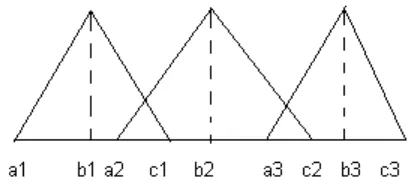
A Fuzzy Controller is characterised by inputs and outputs. The inputs and outputs are correlated by Membership Functions (MF). In this case there are two inputs 1) Error of speed. 2) Change in Error of speed.

2.1

Membership Functions

Each of the inputs have 3 membership functions – for Negative, Zero and Positive. The MFs are chosen to be triangular in shape. There is only one output i.e. Voltage which is fed to the armature of the DC Motor . The Voltage also has 3 MFs – Negative, Zero, positive but it is not required to be optimised. Since the input to the fuzzy controller deals with the quantity to be controlled only the Input MF is sufficient to be optimised. Mamdani (Fuzzy inference System) FIS has been used. For each triangular membership function there are 3 parameters a,b,c. Since there are 3 MFs for a particular input there are a total of 9 parameters for a particular input. Since there are 2 inputs so there are a total of 18 parameters for each input. The membership functions of one input is shown.

Fig 1: Membership Functions and their Parameters

38 objective function for PSO should be a function of output of

the fuzzy controller. The details of how the objective function is found out is given in the next section. Now discussion will be on the PSO algorithm[3]. The PSO search space is multidimensional. The dimension is determined by the number of variables whose value we are to find. In this case the dimension is 8. A point in the space is referred to as a particle. Each particle moves in the search space with a velocity dependent on its own flying experience and it’s companions’ flying experience. Each particles keeps a note of its best solution (best evaluating value of the objective function) which is termed as personal best (pbest). The global best (gbest) is the best solution in the whole group. In each iteration the velocity and the position is updated according to the following rule[4].

2.2 PSO Variables

For example let the jth particle be represented by xj=

(xj1,xj2,xj3,...xjg) in the g dimensional space. The best previous

position of the jth particle is pbestj=(pbestj1,pbestj2,...pbestjg).

The best particle corresponds to gbestg. The velocity of the

particle j is represented as vj=(vj1,vj2,...vjg). The new velocity

and new position for a particular iteration k+1 is as : vjg(k+1)=w.vjg(k)+c1*rand()*(pbestjg–xjg(k))

+c2*rand()*(gbestg – xjg(k))

xjg(k+1) = xjg(k)+vjg(k+1)

j=1,2...n g=1,2,...m where

n number of particles in a group m number of members in a particle

k iteration number

v velocity

x particle co-ordiante

c1,c2 acceleration constant normally set to 2 w inertia weight factor

rand() random number between 0 and 1

In this way the particle moves about in space and for each iteration it checks for the optimization of the objective function. The next section will be about the working model and the implementation of the algorithm.

3.

SIMULINK MODEL AND THE

ALGORITHM

The SIMULINK model[5][6] used is given in Fig 2. As can be seen the error and rate of change of error of speed has been normalized and is fed into the fuzzy controller as Input [7]. The Minor Feedback loop in the model is that of a Armature Controlled DC Motor. Hence, the input of the Minor Feedback loop is the Armature voltage which is also the output of the Fuzzy controller. The Minor Feedback path is that of the Back EMF of the DC Motor. The Output MF parameters need not be optimized. The objective function F(i)=0.5 – Output of the Fuzzy Controller. The output of the Fuzzy controller has been evaluated using the evalfis() of MATLAB[8]. The value 0.5 has been calculated as per the set point speed of 23 SI Units. Using the equation E=K*N putting N=23 SI we get E as 0.5 and since the normalisation constant (in the SIMULINK Block diagram) is unity. The constant load torque has been assumed for the motor and shown by the input to the second summer in the minor loop.

Description of the algorithm for tuning the fuzzy controller[9]:

1) The no. of particles (n) is to be 30. The number of iterations (i) is 20.

2) Since 8 variables need to be optimised therefore the paricle is 8 dimensional.

3) For each particle (1 to 30) the following is done: a) The particle’s position i.e. the parameters of

MFs is initialized using the rand(). For e.g. rand(1) gives a random number between 0 and 1. -1+rand(1)*2 gives random number between -1 and +1. So the lower and upper boundaries of the search space are also set in this way. Thus the constraints on the MF parameters can be set

b) The particle’s best known position is initialized to initial position.pi < - xi

c) If F(pi)<F(g) the swarm’s global best position

is updated g < - pi

d) The initial velocity is set to 0.

4) Until i>20 or minimum error tolerance has been achieved the following is repeated :

a) For each particle (1 to 30) :

(i) For each dimension (1 to 8) :

 Velocity of each particle is calculated and updated (ii) The particle’s position is also

updated b) If F(xi)< F(pi)

(i) Update the particle’s best known position pi < - xi

(ii) If F(pi)<F(g) the swarm’s best

known position is updated: g < - pi

5) The M-File where the algorithm is encoded is executed

6) Hence, the optimum values of the 8 parameters are found and fed into a matrix. The other fixed values are clubbed with it to form a 6 X 3 Matrix. 7) The Matrix is fed into the FIS Structure using the

function setfis().

8) The FIS Structure is uploaded into the SIMULINK Fuzzy controller block and then the Model is Simulated.

pi positon vector of personal best g position vector of global best xi postion vector of a particle

i iteration index

For the Set points of 25 and 30 SI the objective function is calculated using the equation described. For Set Point 25 E=0.543 and objective function F(i F(i)=0.543 – Output of the Fuzzy Controller. For Set Point 30 E=0.543 and objective F(i)=0.652 – Output of the Fuzzy Controller. So in the algorithm the objective function is changed for each set point in the way mentioned above. Accordingly results are obtained as shown in the next section.

4.

RESULTS

Results are obtained for two cases firstly by keeping the set point constant and then varying the set point.

4.1

Fixing Set Point

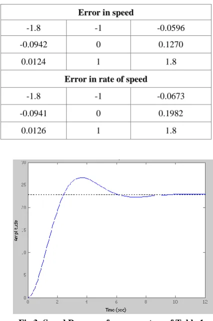
The set point of the speed is set to 23 SI units and the PSO code is executed two times. Therefore two transient responses are obtained with negligible steady state error. As expected oscillations occur because the presence of inductance in armature circuit has been assumed. So the following tables and graphs are plotted.

Table 1. Parameters for setpoint 23 SI Units for first PSO execution

Error in speed

-1.8 -1 -0.0596

-0.0942 0 0.1270

0.0124 1 1.8

Error in rate of speed

-1.8 -1 -0.0673

-0.0941 0 0.1982

0.0126 1 1.8

Fig 3: Speed Response for parameters of Table 1

Table 2. Parameters for Set Point 23 SI Units for second PSO execution

Error in speed

-1.8 -1 -0.0673

-0.0942 0 0.1274

0.0945 1 1.8

Error in rate of speed

-1.8 -1 -0.0274

-0.0339 0 0.0367

40 Fig 4: Speed Response for parameters of Table 2

4.2

Varying Set Point

Now the PSO algorithm is run for different set point. Only single execution of the algorithm is used for the two set points of 25 and 30 SI Units. The results obtained are given below.

Table 3. Parameters for Set point 25 SI Units

Error in speed

-1.8 -1 -0.0396

-0.218 0 0.1345

0.0745 1 1.8

Error in rate of speed

-1.8 -1 -0.0890

-0.9800 0 0.4560

0.0345 1 1.8

.

Fig 5: Speed Response for the parmeters of Table 3

Table 4. Parameters for Set point 30 SI Units

Error in speed

-1.8 -1 -0.0567

-0.0630 0 0.1296

0.1143 1 1.8

Error in rate of speed

-1.8 -1 -0.0789

-0.0959 0 0.1279

0.0568 1 1.8

Fig 6: Speed Response for the parameters of Table 4

5.

CONCLUSION

The PSO tuned Fuzzy controller was simulated on the plant. The plant was chosen to be an armature controlled DC Motor with speed being the quantity to be controlled. The algorithm for tuning the paramaters of the membership functions of the Fuzzy controller has been developed. The optimized parameters so obtained is fed into the SIMULINK Block of the fuzzy controller and results obtained for various Cases. Steady error has been made zero. Response is oscillatory because of presence of inductance in armature circuit. Fig. 3 shows the best response with very little overshoot.

6.

ACKNOWLEDGEMENTS

7.

REFERENCES

[1] S.K.Sinha, R.N. Patel, and R. Prasad “Application of GA and PSO Tuned Fuzzy Controller for AGC of Three Area Thermal-Thermal-Hydro Power System” International Journal of Computer Theory and Engineering, Vol. 2, No. 2 April, 2010

[2] Qinghai Bai “ Analysis of Particle Swarm Optimization”, Computer and Information Science, February 2010 [3] Saeed Vaneshani and Hooshang Jazayeri-Rad,

“Optimized Fuzzy Control by Particle Swarm Optimization Technique for Control of CSTR,” World Academy of Science, Engineering and Technology 59 2011

[4] Zwe-Lee Gaing, “A Particle Swarm OptimizationApproach for Optimum Design of PID Controller” IEEE transactions on Energy Conversion, Vol 19, No. 2, June 2004

[5] Dipraj, and Dr. A.K. Pandey, “Speed control of a D.C. Servo Motor By Fuzzy Controller ,” International Journal of Scientific & Technology Research Volume 1, Issue 8, September 2012

[6] Mehmet Cunkas, Omer Aydogdu “ Realization of Fuzzy Logic Controlled Brushless DC Motor Drives using MATLAB/SIMULINK”, Vol.15, No.2, 2010

[7] J.V. de Oliviera “Semantic Constraints for membership function optimization”, IEEE transactions on Systems, Man and Cybernetics, January 1999

[8] R.N. Patel, S.K.Sinha, and R. Prasad, “Design of a Robust Controller for AGC with Combined Intelligence Techniques,” World Academy of Science, Engineering and Technology 21 2008