Managing Communication Delays and Model Error
in Demand Response for Frequency Regulation
Gregory S. Ledva,
Student Member, IEEE,
Evangelos Vrettos,
Student Member, IEEE,
Silvia Mastellone,
G¨oran Andersson,
Fellow, IEEE,
and Johanna L. Mathieu,
Member, IEEE
Abstract—This work develops and compares several networked control and estimation algorithms to manipulate the power consumption of a population of residential thermostatically controlled loads (TCLs) to fulfill PJM frequency regulation re-quests given an imperfect communication network and modeling error. The algorithms rely on a model of the plant to reduce the effects of communication delays, and include a stochastic, predictive controller and two Kalman filter-based state estimation techniques. The first estimator uses a set of independent Kalman filters that run in parallel, and the second incorporates individual TCL models that rely on identified thermal parameters.
We use simulations to examine 1) the algorithms’ ability to adequately provide frequency regulation under a range of delay severities, and 2) the effect of increased modeling error. We find that both estimator-controller combinations provide acceptable frequency regulation with average delays of 20 seconds and minor modeling error. When we increase the modeling error by using a higher-order model to represent the TCLs within the plant, the first estimator provides acceptable frequency regulation while the second estimator provides poor frequency regulation.
Index Terms—Demand response, frequency regulation, delays, state estimation, optimal control, networked control
I. INTRODUCTION
I
NCORPORATING more fluctuating, renewable power gen-eration into the electricity network will usually lead to addi-tional power production variability. To maintain the frequency within an acceptable range, generation resources must supply more reserves, which may require them to operate at inefficient operating points [1]. Alternatively, the manipulation of electric power demand using demand response is also capable of providing frequency regulation.Common residential demand response methods include price-based demand manipulation and direct control of loads [2], e.g., residential thermostatically controlled loads (TCLs) such as air conditioners, heat pumps, and water heaters. Under normal operation, TCLs cycle on and off to maintain the temperature of an internal medium, e.g., a house’s air temper-ature, around a user-defined set-point. Direct control strategies manipulate a TCL population’s total power demand generally by adjusting either the user-defined temperature set-point, e.g., [3]–[5], or by requesting additional on/off switching, e.g., [6]– [8]. Aggregations of TCLs can be used to provide ancillary services such as frequency regulation to the power system [5]. Recently, researchers have developed non-disruptive load
G. S. Ledva and J. L. Mathieu are with the Department of Electrical Engi-neering & Computer Science, University of Michigan, Ann Arbor, MI 48109 USA (e-mail: [email protected]; [email protected]). E. Vrettos and G. An-dersson are with the Power Systems Laboratory, ETH Zurich, 8092 Zurich, Switzerland (e-mail: [email protected]; [email protected]). S. Mastellone is with the Corporate Research Center, ABB, 5405 Baden-D¨attwil, Switzerland (e-mail: [email protected]).
control strategies [9], ensuring TCLs operate within or very close to their normal temperature range [5].
TCLs are a spatially distributed resource, and coordinating the demand of thousands of them to provide frequency regula-tion requires sensing and communicaregula-tion infrastructure. This infrastructure enables TCLs to receive control inputs and to send information about their current operating state. However, the cost of this infrastructure can be prohibitive [10]. Using existing infrastructure, such as smart meters, is possible but the frequency of information retrieval is limited [11], and load control input delays can be significant [12]. Developing control algorithms for demand response that are robust to delays and respect the limitations of existing infrastructure may lower the cost of demand response implementations.
Networked control theory addresses imperfect communica-tion within control systems, see e.g., [13]. Ref. [14] investi-gates the impact of delays in frequency regulation including batteries and develops control algorithms to limit their effects. Within the demand response literature, [6]–[8], [15], [16] develop control strategies to address infrequent or unavailable state measurements, [17] investigates lost messages in optimal load scheduling, and [18] investigates the impact of, but does not compensate for, communication latencies.
In this paper, we develop non-disruptive control and estima-tion algorithms that enable aggregaestima-tions of residential TCLs to provide ancillary services such as frequency regulation (i.e., secondary frequency control) in the presence of significant communication system limitations, including delays, as well as substantial error within the model used by the algorithms. In practice, we would expect large model mismatch since it is difficult to develop a computationally-tractable and accurate model of the aggregate dynamics of large number of spatially-distributed, heterogeneous TCLs, especially given that many useful TCL parameters and states are not easy to measure.
Our primary contribution is to adapt networked state esti-mation and control approaches so to that they can be used to solve key practical problems that will be encountered in cost-effectively coordinating large numbers of heterogeneous distributed TCLs for ancillary services. We propose two state estimation strategies, one that synthesizes estimates obtained from a bank of Kalman filters acting on non-synchronous state measurements and another that uses individual TCL state predictions obtained from identified TCL models as pseudo-measurements within a single Kalman filter. We also propose a model predictive control (MPC) algorithm that uses a probabilistic estimate of the control input.
State Estimator Controller
Aggregator
State Estimate
Input Estimate State Estimator
State Estimator Controller
Aggregator
State Estimate
Input Estimate State Estimator
Desired Aggregate TCL Demand
Plant
Communication Network
...
SubstationTCL 1 TCL 2
Uncontrollable Loads
...
Total Demand Measurement
Broadcast Input TCL Measurement
Histories
Delayed Total Demand
Measurement
IID Delayed TCL Measurement
Histories
[image:2.612.53.295.56.243.2]IID Delayed Inputs TCLNTCL
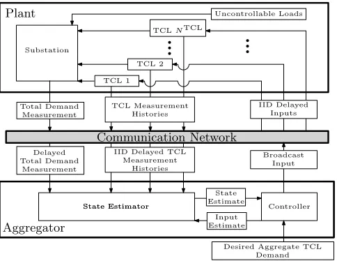
Fig. 1. An overview of the control framework.
proposed in [19]; 2) we track real PJM frequency regulation signals (rather than simple sinusoidal signals as in [19]) to evaluate the impact of delays on the adequacy of the frequency regulation from demand response; 3) we evaluate the control and estimation algorithms in tandem (rather than individually as in [19]); 4) we evaluate the impact of modeling error by testing the algorithms on a more realistic simulated plant, and compare the results to those generated with the simpler plant used in [19]; 5) we find that both estimator-controller combinations can effectively mitigate communication delays; and 6) we find that one estimator is sensitive to the specific model used in the plant whereas the other is not.
The remainder of the paper is organized as follows: Sec-tion II describes the problem framework. SecSec-tion III presents individual and aggregate TCL models. Section IV develops two state estimation algorithms that we use in conjunction with a control algorithm that Section V develops. Section VI formulates a number of case studies and presents their results. Finally, Section VII discusses the conclusions.
II. PROBLEMFRAMEWORK
As shown in Fig. 1, we assume a problem framework that contains a plant, a communication network, and an aggregator. The plant consists of a set of NTCL controllable TCLs, some
uncontrollable loads, and a distribution substation that serves the total demand of the plant. We assume a smart meter acts as an interface between each TCL and the communication network, allowing two-way communication between the TCLs and the aggregator through an imperfect communication net-work as in [8].
We make several assumptions regarding the communication network and smart meters. Due to the capabilities of digital communication networks, we assume that multiple measure-ments and inputs can be transmitted within one communication packet, i.e., message. We also assume the messages are time-stamped [13] and the clocks are synchronized across the com-munication network nodes, allowing knowledge of previously realized delays and their resulting statistics. We assume that the communication network imposes independent and identi-cally distributed (IID) delays on each message. We assume the
smart meter can use logic to select an applicable input from a set of inputs, as explained in Section V. Finally, we assume each smart meter can collect histories of the TCL’s internal air temperature and on/off mode measurements, but the smart meter can only transmit these state measurement histories infrequently, e.g., every fifteen minutes, due to communication limitations as in [8].
We assume the aggregator, which acts as a central controller, uses a state estimator and controller, both of which include a model of the plant. The aggregator induces TCL on/off switch-ing by broadcastswitch-ing inputs at each time-step (every two sec-onds). The inputs are designed to produce a desired aggregate TCL demand and are described in more detail in Section III-B. IID delays cause the inputs to arrive asynchronously, and so an estimated input is used by the aggregator. We assume that the desired aggregate demand values are frequency regulation signals, e.g., automatic generation control (AGC) or secondary frequency control signals, provided by the system operator.
The aggregator’s state estimation algorithm produces an estimate of the TCL aggregation’s state, which is described in Section III-B. We assume that the aggregator has access to measurements of the total substation demand and TCL state measurement histories as in [8]. As in [8], substation demand measurements are available at every time-step, and the aggregate TCL demand is estimated from these measurements by subtracting a prediction of the uncontrollable load. While the substation demand measurements may be accurate, errors in predicting the uncontrollable demand result in measurement noise on the aggregate TCL demand. In this work, we add normally-distributed, zero-mean noise to the aggregate TCL demand to approximate the prediction error and any noise in the substation demand measurements. As in [8] the TCL measurement histories are available infrequently (every 15 minutes) due to smart meter limitations.
The infrequent availability of possibly delayed TCL state measurements, means the aggregator relies on output feedback (i.e., the aggregate TCL demand estimates, referred to as “aggregate power measurements”) at most time-steps to form the state estimate. The state estimate is then used by the aggregator to generate the control inputs.
III. MODELING
We use three previously developed models and describe them here for completeness and to establish the notation used throughout the paper. Two hybrid, heat- transfer-based models represent individual TCLs, and a Markov chain model represents the TCL population.
TABLE I TCL MODELPARAMETERS
Parameter Description Three-StateValue Two-StateValue
θset Temperature Set-Point [◦C] [23, 25] [23, 25] θdb Temperature Deadband [◦C] [0.85,1.15] [0.85,1.15]
θo Outdoor Temperature [◦C] 32 32 Um Envelope Conductance [kW◦C] [4.35, 5.87]
-Ua Internal Conductance [kW◦C] [0.26, 0.35] [0.41, 0.56]
Λm Mass Heat Capacitance [kWh◦C] [1.93, 2.60]
-Λa Air Heat Capacitance [kWh◦C] [0.48, 0.64] [0.51, 0.70]
Qm TCL Mass Heat Gain [kW] 0
-Qa TCL Air Heat Gain [kW] N(0, ) N(0, )
Variance forQa[kW2] 2.5E-7 2.5E-7 Qh TCL Heat Transfer [kW] [-16, -12] [-16, -12]
η Coefficient of Performance [-] 3 3
∆t Time-Step Duration [s] 2 2
The hybrid nature of these models, i.e., their usage of both discrete and continuous states, makes it computationally challenging to incorporate thousands of the models within optimization-based control algorithms. The Markov chain model, developed in [6] and referred to as the aggregate model, is a linear model of the TCL population’s power demand dynamics, and it is easily incorporated into control algorithms. The algorithms in Sections IV and V use this aggregate model. The following section describes the individual TCL models, and Section III-B describes the aggregate model. Note that we assume model parameters are time-invariant throughout, but the models can incorporate time-varying parameters. Time-varying parameters within the individual TCL models would result in a time-varying aggregate TCL population model. Assuming that the time-varying aggregate model is known, all of the algorithms are still applicable.
A. Individual TCL Models
We first present a generic discrete-time state update equation for cooling TCLs below, then detail the difference between the two individual models in the following sections. Table I summarizes the model parameters where[α, β]corresponds to
a uniform distribution and N(α, β) corresponds to a normal
distribution with mean αand varianceβ.
Denote the set of TCLs JTCL =
1,2, . . . , NTCL . Each
TCL j ∈ JTCL has continuous-time matrix parameters Ac,j, Bc,j, and Ec,j, and the discrete-time matrix parameters Aj, Bj, and Ej are formed using [24, p. 315]. The vector θtj
denotes the continuous states, which are the TCL’s internal temperature(s) at time-step t. The discrete state corresponds
to the scalar on/off mode mjt, anddjt is a disturbance vector.
The discrete-time state-update equations are
θjt+1=Ajθjt+Bjmjt+Ejdjt j∈ JTCL (1a)
mjt+1=
0 ifθta,j+1< θset,j−θdb,j/2 1 ifθta,j+1> θset,j+θdb,j/2 mjt otherwise,
j∈ JTCL (1b)
where (1a) updates the internal temperatures, (1b) updates the on/off mode, andθa,jt is the element ofθtj that corresponds to
the TCL’s air temperature, which is being regulated. The power demand of TCLj isPtj= (|Qh,j|mjt)/ηj withQh,j <0 for
cooling TCLs. The output of the TCL model, or the values that can be measured, is ytj=
θta,j mjt>.
1) Three-State Individual TCL Model: We use this model to represent individual TCLs within the plant during the case studies presented in Section VI. In the three-state model
θjt =
θa,jt θm,jt >whereθtm,j denotes the TCL’s mass
tem-perature. The disturbance vector isdjt=
θo Qat,j Qm,j>,
where the heat injections Qa,jt and Qm,j arise due to solar
irradiance and heat gain within the household due to occu-pants and additional appliances. The model’s continuous-time matrices are
Ac,j =
− Ua,j+Um,j
/Λa,j Um,j/Λa,j Um,j/Λm,j −Um,j/Λm,j
Bc,j =
Qh,j/Λa,j 0> Ec,j =
Ua,j/Λa,j 1/Λa,j 0 0 0 1/Λm,j
[image:3.612.342.535.174.242.2].
Table I’s “Three-State Value” column parameterizes a popula-tion of residential air condipopula-tioners using nominal parameters from [25]. However, we set the outdoor temperature θo to
simulate a reasonably hot day, we assume Qa,jt is zero-mean
and normally-distributed to include random air temperature disturbances as in [19], and we set Qm,j = 0. The results in
Section VI-B include a discussion of the algorithms’ ability to accommodate positively biased heat injections.
2) Two-State Individual TCL Model: We use these mod-els within the estimator described in Section IV-B2. In the two-state model θjt = θta,j and djt =
θo Qat>
. The resulting continuous-time matrices are Ac,j = −Ua,j/Λa,j, Bc,j = Qh,j/Λa,j and Ec,j =
Ua,j/Λa,j 1/Λa,j
. We set the parameters in Table I’s “Two-State Value” column equal to the three-state model values where applicable, but we set
Ua,j andΛa,j such that the nominal cycle time is comparable
to that of the three-state model.
B. Aggregate TCL Population Model
The aggregate model, which is used by the controller and estimator, assumes that the two-state model of Section III-A2 is the underlying individual TCL model. While an aggregate model exists for the three-state TCL model [5], measurements of θm,jt are not easy to obtain, and practical construction
of the state-transition matrix from available measurements is an open question. In Section VI, we evaluate the impact of this assumption on the control and estimation algorithms’ performance by simulating TCLs within the plant using the three-state model.
The aggregate model uses an aggregate state xt ∈ RN x
whereNxis the number of discrete states, and each element of
the state vector corresponds to the portion of TCLs within the discrete state. The discrete states are formed by first defining a normalized temperature deadband and then dividing it into
Nx/2temperature intervals. Each interval contains two states –
one for TCLs that are drawing power and one for TCLs that are not. The state transition matrixA∈RN
x×Nx
is a transposed Markov Transition Matrix that describes the probability of TCLs transitioning between states in a time-step.
The input ut ∈ RN x/2
B ∈ RNx/2×Nx ensures the TCLs are forced into the
oppo-site on/off bin within the same temperature interval. Before transmitting input vectors to the TCLs, this input is converted into a switching probability by normalizing each input element with the corresponding state element. To implement these switching probabilities, each TCL first selects the probability corresponding to its current state. Then, each TCL determines whether it switches by drawing a random number. We assume the local TCL controller disregards switching requests when necessary to maintain the temperature within the normal operating range.
The output of the aggregate model yt depends on whether
both aggregate state and aggregate power measurements are available at time-stept. The setTSdenotes time-steps where both aggregate state and aggregate power measurements are available, andyt∈RN
x+1
at these time-steps. Otherwise only aggregate power measurements are available andyt∈R. The
resulting linear system is
xt+1=Axt+But+wt (3a)
yt=
CPxt+vPt t /∈ TS "
CS CP #
xt+ "
vSt vPt #
t∈ TS, (3b)
where wt ∈ RN x
is process noise including modeling error,
vSt ∈RN x
is the aggregate state’s measurement noise,vPt ∈R
is the aggregate power’s measurement noise,CSis anNx×Nx
identity matrix,CP=PonNTCL[0 · · · 0|1 · · · 1], andPon is
an approximation for the average power draw of a TCL that is on within the aggregation. We calculate Pon using data from
a setThistofNhisthistorical time-steps when the TCLs cycled
without external forcing
Pon= 1 Nhist
X
t∈Thist
P
j∈JTCL
Ptj
P
j∈JTCL
mjt
. (4)
The quantity P
j∈JTCLPtj is the total power draw of TCLs
at time-step t, and P
j∈JTCLmjt is the number of TCLs that
are on at time-step t. Finally, we assume that the aggregate
model is known to the aggregator a priori. It can be derived or identified using the methods in [6].
IV. STATEESTIMATIONALGORITHMS
Our state estimation algorithms use a networked, time-varying Kalman filter from [26] that incorporates aggregate state and power measurements. The networked Kalman filter excludes measurements that have not arrived from the cal-culations at each time-step using binary indicator variables. As delayed measurements arrive, the networked Kalman filter fully incorporates the new information by updating a history of estimates. Measurement delays are treated deterministically within the estimator since delays associated with measure-ments that have arrived are known. Whereas [26] does not include inputs within the estimator’s dynamic model, we use estimated inputs that are described in Section V-B.
To incorporate delayed measurements, past estimator values must be stored so that they can be updated. The memory
requirement can be reduced by excluding measurements with delays longer than a preset threshold; for generality, we do not set a delay threshold in this work. Setting a delay threshold within the estimator implies that measurements are discarded if they do not arrive by the deadline. As measurements take longer to arrive, their information becomes outdated and they are less useful. The threshold can be set given the known delay statistics such that only a small number of measurements are discarded due to late arrival and the impact on the state estimate is small. Section IV-A presents the networked Kalman filter, and Section IV-B presents two variations of it, which we apply to our problem.
A. The Networked Kalman Filter
Within this section and Section V, we use the time indexing notation ψk|t where ψ is an arbitrary value, and t denotes
the time of the calculation. In this section, k ≤ t indexes a
historical horizon of time-steps. The horizon lengthNtkfis set
at each calculation timet as the number of time-steps of the
newly-arrived measurements’ largest delay, and the set of time-steps within the historical horizon isKtkf=t−Ntkf, . . . , t .
The set Kkft includes past time-steps requiring an update to incorporate the newly arrived measurements into the state estimate, and the present time-step for which a new state estimate must be generated.
The binary, scalar variablesγkS|t and γkP|t indicate whether
the aggregate state and aggregate power measurements sam-pled at time-stepkhave arrived by time-stept. The indicators
are 0 if the corresponding measurement has not arrived by time-step t, and 1 otherwise. The indicator γkS
|t is also set
to 0 when the aggregate state is not measured. The Kalman filter observations incorporate the aggregate state measure-ments ykS and the aggregate power measurements ykP using yk|t=Ck|tx+vk|twhere
yk|t= "
γkS|tykS γkP|tykP #
, Ck|t= "
γkS|tCS γkP|tCP #
, andvk|t= "
γkS|tvSk γkP|tvPk #
.
The measurement noise vk|t has covariance Vk|t, which is a
block diagonal matrix composed of the aggregate state and aggregate power measurement noise covariances γkS|tVS and γkP|tVP. These covariances are assumed to correspond to
zero-mean, normal distributions. The indicator values ensure that measurements that have not arrived have no effect on the state estimate, and the resulting zero components ofyk|t,Ck|t, vk|t, andVk|tcan be removed to reduce the dimension of the
computations with no effect on the estimate. The quantities
e
yk|t,Cek|t,evk|t, andVek|t correspond to the reduced matrices.
To perform state estimation, we initialize the recalculation horizon using the state estimate and error covariance from the calculation at timet−1: bxt−Nkf
t−1|t=xbt−Ntkf−1|t−1 and
Ht−Nkf
t−1|t=Ht−Ntkf−1|t−1. Previous state estimates are then recalculated to incorporate newly arrived measurements, and a new state estimate is generated for time-step k = t. For k∈ Kkft:
b
x−k|t=Axbk−1|t+Bbuk−1 (5a) Hk−
Kk|t=Hk−|tCek>|t
e
Ck|tHk−|tCek>|t+Vek|t †
(5c)
b
xk|t=xb−k
|t+Kk|t
e
yk|t−Cek|txb−k
|t
(5d)
Hk|t=Hk−|t−Kk|tCek|tHk−|t. (5e)
The aggregate model in (5a) generates an a priori state pre-dictionxb
−
k|tand error covarianceHk−|tin (5b), whereW is the
process noise covariance of a zero-mean, normal distribution. Section V explains the estimated inputbuk in more detail. The
Kalman gain Kk|t is calculated in (5c) based on available
observation values with † denoting a pseudo-inverse, which we use for numerical reasons. The a posterioristate estimate
b
xk|tand error covarianceHk|tare then calculated in (5d) and
(5e). The output of the algorithm is the new state estimate for the current time-stept, i.e.,xbt=xbt|t, which fully incorporates
all measurements that have arrived. Note that the process noise is not necessarily zero-mean and normally-distributed, which results in a sub-optimal filter. We assume that the measurement noise and process noise are independent from each other and independent in time.
B. Variations of the Networked Kalman Filter
Because of IID transmission delays, the state measurement histories from individual TCLs do not arrive synchronously at the aggregator. We develop and investigate the performance of two methods to form aggregate state estimates from asyn-chronous TCL measurements for use within the networked Kalman filter. The method in Section IV-B1 describes an algorithm that runs NTCL filters from Section IV-A, one
for each TCL. The method in Section IV-B2 uses a single networked Kalman filter that uses aggregate state predictions obtained by applying identified individual TCL models to old state measurements. Both methods use (delayed) aggregate power measurements that are sampled at every time-step and (delayed) TCL state measurements that sent to the aggregator infrequently, e.g., every fifteen minutes.
1) Estimator 1: Parallel Kalman Filter Estimator: An ag-gregate state measurement can be formed using each TCL’s state measurement, i.e., its temperature and on/off mode measurements, and used within a networked Kalman Filter. However, this would require waiting until all TCL state mea-surements have arrived at the aggregator, and so the aggregate measurement delay would be equal to the worst-case TCL state measurement delay. Instead, we construct a state estimator that runs NTCL networked Kalman filters in parallel, one
for each TCL. When a TCL state measurement arrives, we use it within the corresponding Kalman filter and combine all filter estimates into a single aggregate state estimate. By doing this, we can update the aggregate state estimates while measurements are still arriving.
Each of the filters use the aggregate model, delayed ag-gregate power measurements, and delayed TCL state mea-surements from the corresponding TCL. While TCLs transmit measurement histories, only the most recent measurement is used in this method. We define the state vector of each filter as xjt ∈ RN
x
for j ∈ JTCL; it is defined equivalently to
xt in Section III-B, however xjt models a single TCL. To
form xjt, we convert TCL j’s most recent air temperature
and on/off value into its corresponding discrete bin value within the aggregate state. We then set the element of xjt
corresponding to the TCL’s discrete bin value to 1 and all other elements to 0. We assume TCL state measurements are accurate for convenience, and so we use a near-zero aggregate state noise covariance, i.e.,VS,j≈0∀j. We use the
the aggregate power measurement noise covariance defined in Section IV-A, and we assume that the covariance of this measurement noise is significantly greater than zero due to errors in predicting the uncontrollable demand as described in Section II. The estimates produced by each filter are combined into an overall aggregate state estimate at each time-step as
ˆ xt =
PNTCL
j=1 xb j t
/NTCL. The main disadvantages of this
method are the large computational requirement of running
NTCL Kalman filters in parallel and the usage of only the
most recent TCL measurements.
2) Estimator 2: Single Kalman Filter Using State Predic-tions: This state estimator consists of three components: an individual TCL parameter identification algorithm, a bank of
NTCLidentified two-state individual TCL models as described
in Section III-A2, and a single networked Kalman filter as described in Section IV-A. The parameter identification algorithm uses the TCL state measurement histories to identify the thermal parameters for each TCL, which we assume are initially unknown to the aggregator. We assume that measure-ments of thermal mass temperature are unavailable, as they would be difficult to obtain in practice. Therefore, we use the two-state individual TCL models, as it would be difficult or impossible to identify the three-state model parameters.
This estimator uses delayed aggregate power measurements and delayed TCL state measurement histories sampled at every time-step but transmitted infrequently, e.g., every fifteen minutes. As each TCL’s measurement history arrives, it is used within a nonlinear least squares algorithm to identify the thermal parameters Λba,j and Uba,j corresponding to the
two-state individual TCL model, assuming that the set-point, deadband width, and outdoor temperature are known. We use the identified models to predict the TCL states at each time-step (assuming Qa,jt = 0∀j), and we use the individual
predictions to form an aggregate state prediction x?t.
A single networked Kalman filter treats the predictions
x?
t as measurements, allowing the individual TCL models to
influence the Kalman filter estimate. The measurement noise associated with the aggregate state predictionsvtS is assumed
to be zero-mean and normally-distributed, and the aggregate state measurement noise covarianceVSis generated using the
historical errors. Note that the noise will not be normally-distributed in general, which results in a sub-optimal filter. As in Section IV-B1, the measurement noise associated with the aggregate power measurements is significant, and so the associated covariance is greater than zero.
The method has the disadvantage that it relies on the accuracy of the two-state model; the implications are discussed in Section VI. This estimator must keep track of and com-pute the state of NTCL two-state models and requires one
amount of information, e.g., matrices and states, that must be stored for each Kalman filter depends on the aggregate model’s dimension Nx. Qualitatively, the data requirements
and necessary computations, i.e., matrix multiplication, for each estimator are similar.
This state estimator consists of three components: a param-eter identification algorithm, a bank of NTCL identified
two-state individual TCL models, and a single networked Kalman filter. As each TCL’s measurement history arrives, they are used within a nonlinear least squares algorithm to identify the thermal parametersΛba,jandUba,j of the TCL, assuming a
two-state TCL model and that the set-point, deadband width, and outdoor temperature are known. The set of identified TCL models allow each TCL to be simulated where we assume
Qa,jt = 0for all j. Aggregate state predictionsx?t are formed
based on model predictions at each time-step.
A single networked Kalman filter treats the predictions
x?t as measurements, allowing the individual TCL models
to influence the state estimator. The measurement noise as-sociated with the aggregate state predictions vSt is assumed
to be zero-mean and normally-distributed, and the aggregate state measurement noise covarianceVS is generated using the
historical errors. Note that the noise will not be normally-distributed in general, which results in a sub-optimal filter. The method has the disadvantage that it relies on the accuracy of the two-state model, which is discussed in Section VI-B.
V. CONTROLALGORITHM
The aggregator uses the predictive control approach de-scribed in [13] to counteract input delays. In this approach, the control algorithm generates an open-loop input sequence
Ut∈RN
x/2×Nmpc
at each time-step based on the current state estimate. IID delays cause asynchronous input arrival at the TCLs. Using time-stamping, we assume that the smart meter (or TCL) can select the most recently generated input sequence that has arrived. The TCL then selects the input from that sequence that applies to the current time-step, or it uses a zero input. The controller does not know the implemented input at each TCL, and an estimated input is generated from the known delay statistics and is used within the aggregator’s algorithms. We develop an MPC algorithm that considers a horizon of
Nmpctime-steps ranging from the present time-steptto future
time-step t+Nmpc−1 to generate Ut. The MPC algorithm
uses the aggregate model to design inputs to track the desired aggregate demand ytP,ref.
Within this section, k is used to indicate the time-step
of the MPC horizon. Inputs corresponding to time-step k
are produced at time t = k−Nmpc + 1, . . . , k, resulting
in a total of Nmpc inputs for each time-step. The matrix
Uk = uk|k . . . uk|k−Nmpc+1 denotes the set of input
vectors that apply to time-stepk.
As in [27], we form an input estimateubtbased on previously
transmitted input sequences. Ref. [27] attempts to estimate the single input within an actuator whereas we form the input estimate but as the weighted sum of possible inputs and their
probability of being implemented. Specifically, we send a finite number of inputs that apply to time-step k to the TCLs.
The inputs are known because the controller designs them.
Using knowledge of the TCLs’ input selection logic and the probability distribution of delays, which is assumed known from historical data, we compute the probability that each of the inputs that applies to time-step k is implemented by
the TCLs, where P is the vector of probabilities. The MPC formulation uses the expected value of the input. This allows us to reformulate the stochastic optimization problem as a deterministic optimization problem [28]. Section V-B details the construction of ubt, Uk, and P. The following section
presents the MPC formulation, which is a finite-horizon, linear quadratic output regulator with input and state constraints that is implemented using [29].
A. MPC Formulation
To set Nmpc, we first fix a parameter pmax. The value 1−pmax is the probability that no valid input is available
at the TCL, and we explain this further in Section V-B. The MPC algorithm is initialized using the current state estimate
xt=bxt, the current aggregate demand request y P,ref
t , and any
previously transmitted inputs that apply to time-steps within the horizon. The full formulation is
minimize
u,δ
t+Nmpc−1
X
k=t h
cy(yerrk )2+cδ(δ−k +δk+)
+ k X
m=k−Nmpc+1
cu(u>k|muk|m)i (6)
s.t. xk+1=A xk+Bubk (7)
b
uk =UkP (8)
yerrk =yP,refk −CPxk (9) uik|m≤xik i∈ {1, . . . , Nx/2} (10) −uik|m≤xkNx+1−i i∈ {1, . . . , Nx/2} (11)
0−δ−k ≤xk≤1 +δk+ (12)
0≤δ−k, δ+k. (13)
The objective function (6) minimizes the total cost over the horizon where the costs cy,cu, and cδ penalize the tracking
errorykerr, control effort, and soft constraint violationsδ+k and δ−k. The input uk|m in (6) is a column ofUk. The dynamic
model in (7) corresponds to (3a) excluding the process noise and using the estimated input from (8). The tracking error is calculated in (9) using a persistent value of the current aggregate demand request, i.e., yP,k ref = ytP,ref for all k in
the MPC horizon. The input constraints (10) and (11) limit the fraction of TCLs to switch from a particular bin to be less than the fraction of TCLs within that bin. The soft state constraint (12) is satisfied regardless of the initial value provided from the unconstrained state estimator, and (13) restricts the soft constraint violations to positive values.
B. Constructing Input Estimates
The vector P weights each of the inputs in Uk based
The inputs in Uk become “older” as we go from left to
right in the matrix, and we calculate the elements of P using the corresponding input vector’s location in Uk. Due to its
input selection logic, a TCL uses the input corresponding to the leftmost column ofUk that has arrived. The probability of
using a column depends on two events: 1) the column must have arrived, and 2) every column to its left withinUkmust not
have arrived. We generate the elements of P based on these two events, the necessary delays for these events to occur, and the probability of realizing these delays. Note that while assuming IID delays simplifies the following calculations, they are still possible without independence.
To simplify the notation in the following discussion, denote the ith element of P as pi, the ith column of Uk as ui
(which was previously denoted uk|k−i+1), the delay in time-steps associated with the arrival of column ui as τi, and the
probability of the first and second necessary events asp1,iand p2,i. The delays take non-negative, integer values. Using the
assumption of IID delays, pi=p1,ip2,i.
We say that the inputui=uk|k−i+1arrives within time-step
k if its delay is less thani
p1,i=p(τi < i) i= 1, . . . , Nmpc. (14)
For example, u1=uk|k arrives within time-stepkif τ1<1,
i.e., τ1 = 0, and u2 = uk|k−1 arrives within time-step k if
τ2<2, i.e.,τ2= 0 orτ2= 1.
The probability that ui has not arrived by time-step k is p(τi ≥ i). Assuming IID delays, the probability that all
columns left of columni have not arrived by time-stepkis
p2,i= i−1
Y
n=1
p(τn ≥n) i= 1, . . . , Nmpc. (15)
For example,u3=uk|k−2can only be used ifu1andu2have not arrived by time-step k, i.e.,τ1≥1 andτ2≥2.
For an MPC calculation, columns within Uk whose right
time index is less thantcorrespond to inputs that have already
been sent to the TCLs. The remaining columns are inputs that the MPC algorithm chooses (i.e., decision variables within the optimization problem (6)–(13)), but only a portion of these are included in the input sequence Ut sent to the TCLs after the
MPC calculation. Specifically, Utconsists of the one column
from each Uk, k ∈ {t, . . . , t+Nmpc−1}, whose right-hand
time index corresponds to the current time t, i.e., everyua|b
withb=t. The horizon lengthNmpc is set such that the sum
of elements inP is greater thanpmaxwhereNmpcis the length
of P.
VI. CASESTUDIES
We summarize a series of simulations investigating 1) the impact of compensating for delays, and 2) the ability of the methods to provide frequency regulation despite communica-tion delays and model error. Seccommunica-tion VI-A details the simula-tion parameters, algorithm combinasimula-tions, delay distribusimula-tions, reference signal construction, and quantities used to evaluate the simulations. Section VI-B presents the simulation results.
TABLE II SIMULATIONPARAMETERS
Parameter Description Value
Nx Number of State Bins [-] 100
NTCL Number of TCLs [-] 10,000
RP Aggregate Power Noise Covariance [kW2] N(0,4E6) Pavg Average Steady-State TCL Demand [kW] 6E3
∆t Time-Step Duration [s] 2
∆tS,s TCL State Measurement Interval [s] 2
∆tS,t TCL State History Transmission Interval [s] 900 nsteps Time-Steps in Simulation [-] 1800
pmax MPC Delay Probability Threshold [-] 0.999
cy MPC Output Cost [-] 1
cu MPC Input Cost [-] 1
cδ MPC Soft Constraint Cost [-] 1.01
A. Case Study Setup
Table II details the simulation parameters. We simulate a TCL population of 10,000 air conditioners. The average steady-state TCL demand is slightly different between the two- and three-state TCL model populations because of the parameters used, and the value in the table is approximate. We use a zero-mean, normal distribution to generate the aggregate power measurement noise. Similar to [6], [19], we set the noise variance assuming the average steady-state TCL demand is 15% of the demand served by the substation, and the standard deviation of the power measurement noise is set to 5% of the total substation load. We generate the aggregate model’s process noise covariance using historical errors. The resulting process noise is neither zero-mean nor normally-distributed.
We conduct a series of case studies, varying: 1) the average delay, 2) the reference signal, 3) the model used to simulate individual TCLs within the plant, and 4) the estimator. The two reference signals, called the Reg-A and Reg-D reference, correspond to segments of published PJM traditional and dynamic frequency regulation signals from [30]. The reference signals are from May 4, 2014. The signals are interpolated to two second time-steps, and each signal is scaled so that the maximum demand change request corresponds to ±20% of
the average steady-state aggregate TCL demand. Three delay distributions are used, referred to by their average delay: 0, 10, and 20 seconds. With average delays of 0, we do not impose any measurement or input delays. With average delays of 10 and 20 seconds, IID delaysτ are sampled from a discretized
log-normal distributionτ=bexp(τ?)cwhereb·crounds down and τ? is normally-distributed. In the cases with delays, the
variance of the log-normal distribution is0.25sec2. We use the chosen distribution to model delays that do not take negative values and are unbounded above. Recall that the estimator treats the delays deterministically after each measurement has arrived, and so the delay distribution does not impact the estimator performance. The controller uses the statistics of the delay distribution, and so alternative distributions would change the entries inP, but these can be computed regardless of the distribution.
We compare four control setups, which vary both the complexity of delay compensation method and the estimator used.
• Estimator 1-FC, where FC refers to “full compensation,”
setup requires measurement and input time-stamping, aggregator knowledge of the input delay statistics, and that TCLs are capable of input selection.
• Estimator 2-FC, pairs the controller from Section V with
Estimator 2. This setup requires measurement and input time-stamping, aggregator knowledge of the input delay statistics, and that TCLs are capable of input selection.
• Estimator 1-TS, where TS refers to “time stamping,” pairs
Estimator 1 with a simplified controller that does not require aggregator knowledge of the input delay statistics, but still requires measurement and input time-stamping. The controller assumes that there are no input delays and sets the probability of the input arriving at the TCL within the time-step to 1, i.e., P = 1. Additionally, it uses only
one time-step within the MPC algorithm, i.e., Nmpc= 1
because this is all that is necessary without delays [31] and the reference signal is unknown in future time-steps. Time-stamping enables measurement delay compensation in the estimator and input selection at the TCLs.
• Estimator 1-NC, where NC refers to “no compensation,”
pairs Estimator 1 with a simplified controller that does not require aggregator knowledge of the input delay statistics and assumes measurements/inputs are not time-stamped. As in Estimator 1-TS, the controller does not account for input delays. Since measurements are not time-stamped, the estimator uses measurements based on their arrival time rather than their sampling time. Since inputs are not time-stamped, TCLs use whichever input arrives first during a time-step or zero if no input has arrived. We quantify the results using two values 1) the normalized RMS tracking error (RMSE), and 2) the PJM score described below. We run ten instances of each case with different realizations of the random quantities and average the RMSE and PJM score across the instances for each case. The RMSE for a single case instance is
PRMSE= 1 Pavg
s 1 nsteps
X
t∈T
ytP,real−ytP,ref
2
(16)
wherePavgis the average steady-state aggregate TCL demand
andyP,realt is the achieved aggregate demand. The PJM score
is a value between 0 and 1 that is calculated using PJM’s standards [32, pp. 52-54]. The score uses the correlation, delay, and difference in energy between the requested and actual signals. A passing score is ≥ 0.75, which could certify a
resource to provide frequency regulation when tracking the PJM test signal. A score of ≥0.50 would be satisfactory to
maintain certification for an arbitrary reference signal.
B. Simulation Results
Figure 2 summarizes the average RMSE for the four control setups, Table III summarizes the average PJM scores, and Fig. 3 provides time series for Estimators 1-FC and 2-FC assuming an average delay of 20 seconds. Note that Fig. 2 does not contain results for cases using Estimator 2-FC and three-state models as the plant. As shown in Fig. 3c and 3d, the resulting RMSE is high (∼15−20%) in these cases, and
we explain the cause below.
0 3 6
Re
g-A
RMSE
(%)
Two-State Plant Three-State Plant
0 10 20
0 3 6
Average Delay (sec.)
Re
g-D
RMSE
(%)
Estimator 1-NC Estimator 1-TS Estimator 1-FC Estimator 2-FC
0 10 20
[image:8.612.331.542.56.242.2]Average Delay (sec.)
Fig. 2. The average RMSE across all simulation scenarios varying the plant (two-state and three-state TCL models), control setup, average delay, and reference (Reg-A and Reg-D). Error bars indicate the range of values achieved across the ten instances of each scenario.
−20
−10
0 10
Demand
Change
(%)
Estimator 1-FC Estimator 2-FC Reference Signal
(a) Two-State Plant, Reg-A Reference
−20
0 20
Demand
Change
(%)
(b) Two-State Plant, Reg-D Reference
−20
0 20 40
Demand
Change
(%)
(c) Three-State Plant, Reg-A Reference
0 0.25 0.5 0.75 1
−200 20 40 60
Time (hr)
Demand
Change
(%)
[image:8.612.322.554.296.523.2](d) Three-State Plant, Reg-D Reference
Fig. 3. Time-series plots comparing the reference tracking of Estimator 1 and Estimator 2 with average delays of 20 seconds.
Note that with no delay, the RMSE and PJM scores of Estimators 1-NC, 1-TS, and 1-FC are all identical in Fig. 2 and Table III since all three methods are equivalent without delay. However, with increasing average delays, the RMSE increases significantly for Estimator 1-NC, increases slowly for Estimator 1-TS, and is roughly constant for Estimator 1-FC. This indicates that i) delay compensation is needed if delays are significant, ii) a simple compensation method reduces the effects of delays, and iii) more complex methods can further mitigate the effects of delays. Estimator 2-FC generally performs worse than Estimator 1-TS, and we discuss this below. Note that all methods produce average PJM scores over the 0.75 threshold, except Estimator 1-NC when used to provide Reg-A with average delays of 10 and 20 seconds.
TABLE III AVERAGEPJM SCORES[-]
Two-State Plant Three-State Plant Control Setup Avg. Delay Reg-A Reg-D Reg-A Reg-D Estimator 1-NC 0 0.852 0.899 0.810 0.894 10 0.727 0.821 0.735 0.835 20 0.707 0.782 0.727 0.805 Estimator 1-TS 0 0.852 0.899 0.810 0.894 10 0.846 0.908 0.821 0.901 20 0.836 0.892 0.801 0.896 Estimator 1-FC 0 0.852 0.899 0.810 0.894 10 0.849 0.908 0.814 0.901 20 0.849 0.903 0.824 0.903 Estimator 2-FC 0 0.785 0.882 —— ——
10 0.799 0.892 —— ——
20 0.807 0.887 —— ——
0 50 100
0 200 400
Bin Number (-)
TCLs
(-)
(a) Two-State Plant
0 50 100
Bin Number (-) (b) Three-State Plant Fig. 4. Comparison of discrete state bin distributions in steady-state for populations of TCLs represented by two-state and three-state models.
while the RMSE is slightly worse for the Reg-D signal. Because the trends are different for each performance metric, it is unclear whether the Reg-A or Reg-D cases are superior. Using the three-state TCL models within the plant resulted in slightly worse RMSE and PJM scores, but they are still above PJM’s threshold, which is important since three-state models capture the TCL dynamics more accurately. While we used zero-mean heat injections to generate all of the results shown in this paper, simulations results (not shown here due to space limitations) indicate that Estimator 1-FC can adequately handle more realistic, biased heat injections. In contrast, Estimator 2-FC is unable to account for biased heat injections.
Estimator 2-FC’s performance is dependent on the TCL model used within the plant. When two-state models are used within the plant, Estimator 2-FC’s PJM scores are acceptable in all scenarios; however, it performs worse than Estimators 1-TS and 1-FC. Estimator 2-FC’s performance is dependent on the number of discrete states Nx, and diminishes ifNx is
reduced, e.g., to 40, for computational reasons. Improvements to Estimator 2-FC may be achievable with more advanced parameter estimation methods.
When the three-state models are used within the plant, Estimator 2-FC is not able to provide effective frequency reg-ulation because Estimator 2 uses two-state models to generate aggregate state predictions, which are treated as measurements within the state estimator. Figure 4 shows the steady-state distribution of TCLs within 100 discrete state bins using the and three-state plants. The distribution in the two-state plant (left) is fairly flat across the first 50 bins, which correspond to TCLs that are off. Alternatively, the distribution in the three-state plant (right) has a large concentration of TCLs around bin 50, which corresponds to the edge of the deadband. This qualitative difference in their distributions means that the two-state models used in Estimator 2 cannot effectively predict the aggregate state when the plant consists
of three-state models. Because the thermal mass temperature and environmental heat injections are difficult to measure, identifying the three-state model is difficult.
VII. CONCLUSIONS
In this paper, we developed a predictive controller and two estimators to mitigate the effects of communication delays within a residential demand response scenario. In simulations, we investigated the ability of the algorithms to control an aggregation of TCLs to track frequency regulation signals. Results show that both estimator-controller combinations are able to effectively provide frequency regulation with average delays of up to 20 seconds. The first estimator, which includes only an aggregate model and relies on a number of Kalman filters running in parallel is effective with both structural-and parameter-based modeling error. The second estimator assumes a specific TCL model and identifies parameters for those models. It is effective if the assumed TCL model structure matches the true model structure.
Future work should incorporate and address time-varying outdoor temperatures and time-varying, biased heat injections into the individual TCL models. Investigating a more effective parameter identification algorithm may allow Estimator 2 to be used in a wider range of scenarios. Modifying the controller to account for modeling error may improve tracking performance. Finally, accounting for non-normally-distributed measurement noise should be investigated.
ACKNOWLEDGMENT
This research was partially supported by NSF Grant ECCS-1508943.
REFERENCES
[1] G. Strbac, “Demand side management: Benefits and challenges,”Energy Policy, vol. 36, no. 12, pp. 4419–4426, 2008.
[2] P. Siano, “Demand response and smart grids – A survey,”Renewable and Sustainable Energy Reviews, vol. 30, pp. 461–478, 2014.
[3] D. S. Callaway, “Tapping the energy storage potential in electric loads to deliver load following and regulation, with application to wind energy,”
Energy Conversion and Management, vol. 50, no. 5, pp. 1389–1400,
2009.
[4] S. Bashash and H. Fathy, “Modeling and control of aggregate air conditioning loads for robust renewable power management,” IEEE Transactions on Control Systems Technology, vol. 21, no. 4, pp. 1318–
1327, 2013.
[5] W. Zhang, J. Lian, C.-Y. Chang, and K. Kalsi, “Aggregated modeling and control of air conditioning loads for demand response,” IEEE Transactions Power Systems, vol. 28, no. 4, pp. 4655–4664, 2013.
[6] J. Mathieu, S. Koch, and D. Callaway, “State estimation and control of electric loads to manage real-time energy imbalance,”IEEE Transactions on Power Systems, vol. 28, no. 1, pp. 430–440, 2013.
[7] T. Borsche, F. Oldewurtel, and G. Andersson, “Minimizing commu-nication cost for demand response using state estimation,” in IEEE PowerTech – Grenoble, 2013.
[8] E. Vrettos, J. L. Mathieu, and G. Andersson, “Control of thermostatic loads using moving horizon estimation of individual load states,” in
Power Systems Computation Conference, 2014.
[9] D. S. Callaway and I. A. Hiskens, “Achieving controllability of electric loads,”Proceedings of the IEEE, vol. 99, no. 1, pp. 184–199, 2011.
[10] SCE, “Southern California Edison company 2012-2014 demand re-sponse program portfolio,” Southern California Edison, Tech. Rep. Ap-plication No. A.11-03-003 filed before the Public Utilities Commission of California, March 2011.
[12] J. H. Eto, J. Nelson-Hoffman, E. Parker, C. Bernier, P. Young, D. Shee-han, J. Kueck, and B. Kirby, “The demand response spinning reserve demonstration–measuring the speed and magnitude of aggregated de-mand response,” in 45th Hawaii International Conference on System Science, 2012.
[13] L. Zhang, H. Gao, and O. Kaynak, “Network-induced constraints in networked control systems – A survey,”IEEE Transactions on Industrial Informatics, vol. 9, no. 1, pp. 403–416, 2013.
[14] K. Wada and A. Yokoyama, “Load frequency control using distributed batteries on the demand side with communication characteristics,” in
IEEE PES Conference on Innovative Smart Grid Technologies, Oct 2012.
[15] A. Ghaffari, S. Moura, and M. Krstic, “Modeling, control, and stability analysis of heterogeneous thermostatically controlled load populations using partial differential equations,”ASME Journal of Dynamic Systems, Measurement, and Control, vol. 137, no. 10, 2015.
[16] J. H. Braslavsky, C. Perfumo, and J. K. Ward, “Model-based feedback control of distributed air-conditioning loads for fast demand-side ancil-lary services,” inIEEE Conference on Decision and Control, 2013, pp.
6274–6279.
[17] N. Gatsis and G. B. Giannakis, “Residential load control: Distributed scheduling and convergence with lost AMI messages,”IEEE Transac-tions on Smart Grid, vol. 3, no. 2, pp. 770–786, 2012.
[18] H. Hao, B. M. Sanandaji, K. Poolla, and T. L. Vincent, “Frequency reg-ulation from flexible loads: Potential, economics, and implementation,” inAmerican Control Conference, 2014, pp. 65–72.
[19] G. S. Ledva, E. Vrettos, S. Mastellone, G. Andersson, and J. L. Mathieu, “Applying networked estimation and control algorithms to address communication bandwidth limitations and latencies in demand response,” in Hawaii International Conference on System Sciences,
2015, pp. 2645–2654.
[20] R. C. Sonderegger, “Dynamic models of house heating based on equivalent thermal parameters,” Ph.D. dissertation, Princeton Univ., NJ., 1978.
[21] N. Wilson, B. Wagner, and W. Colborne, “Equivalent thermal parameters for an occupied gas-heated house,”ASHRAE Transactons, vol. 91, no.
CONF-850606, 1985.
[22] S. Ihara and F. C. Schweppe, “Physically based modeling of cold load pickup,”IEEE Transactions on Power Apparatus and Systems, no. 9,
pp. 4142–4150, 1981.
[23] C.-Y. Chong and A. Debs, “Statistical synthesis of power system functional load models,” inIEEE Conference on Decision and Control,
1979, pp. 264–269.
[24] K. Ogata, Discrete-time control systems. Prentice Hall Englewood
Cliffs, NJ, 1995, vol. 2.
[25] (2015) Gridlab-D House Class Documentation. Online. [Online]. Available: http://gridlab-d.sourceforge.net/wiki/index.php/House [26] L. Schenato, “Optimal sensor fusion for distributed sensors subject to
random delay and packet loss,” inIEEE Conference on Decision and Control, 2007, pp. 1547–1552.
[27] J. Fischer, A. Hekler, and U. D. Hanebeck, “State estimation in net-worked control systems,” in15th International Conference on Informa-tion Fusion (FUSION), 2012, pp. 1947–1954.
[28] A. Shapiro and A. Philpott, “A tutorial on stochastic programming,”
Manuscript. Available at www2. isye. gatech. edu/ashapiro/publications. html, vol. 17, 2007.
[29] J. L¨ofberg, “Yalmip : A toolbox for modeling and optimization in MATLAB,” inProceedings of the CACSD Conference, Taipei, Taiwan,
2004. [Online]. Available: http://users.isy.liu.se/johanl/yalmip [30] PJM. (2015) Ancillary Services. reg-data-external-may-2014.xls.
[Online]. Available: https://www.pjm.com/markets-and-operations/ ancillary-services.aspx
[31] S. Koch, J. L. Mathieu, and D. S. Callaway, “Modeling and control of aggregated heterogeneous thermostatically controlled loads for ancillary services,” inPower Systems Computation Conference, 2011.
[32] PJM Manual 12: Balancing Operations, PJM, 2014, revision 31.
Gregory S. Ledva(S’16) received the B.S. degree in mechanical engineering
from the Pennsylvania State University, State College, PA, USA, in 2010. He received the M.S. degree in energy science and technology at ETH Z¨urich (Swiss Federal Institute of Technology) in 2014. He is currently a Ph.D. candidate in the Department of Electrical Engineering and Computer Science at the University of Michigan, Ann Arbor, MI, USA. His research interests include modeling, estimation, control, and optimization of distributed energy
resources as well as the adaptation of machine learning algorithms for control applications.
Evangelos Vrettos(S’09) received the Dipl.-Ing
de-gree in electrical and computer engineering from the National Technical University of Athens (NTUA), Greece, in 2010. After his graduation, he worked as a research assistant at the Electric Machines and Power Electronics Laboratory of NTUA. In 2016 he received the Ph.D. degree from ETH Zurich (Swiss Federal Institute of Technology), Switzerland, where he worked at the Power Systems Laboratory. Since December 2016 he is a home energy systems engi-neer at the smart-grid laboratory of the Swiss utility company EKZ. His research interests include control theory and optimization methods to enable efficient demand response programs for integration of renewable energy sources in the power system. He is also interested in energy storage technologies and energy-efficient control of buildings.
Silvia Mastelloneis Professor for Control and
Sig-nal Processing at the University of Applied Science Northwestern Switzerland (FHNW). She obtained her Ph.D. degree in Systems and Entrepreneurial En-gineering from the University of Illinois at Urbana-Champaign in 2008. From 2008 to 2016 she was Principal Scientist at ABB Corporate Research Cen-ter in Baden, Switzerland, where she led research projects in the area of advanced control for energy systems. She was a visiting researcher at the Institute of Automation, ETH Zurich, and the Xerox Park Innovation Group. Her research interests include decentralized control and estimation and networked control systems, with applications in power elec-tronics converters, traction systems, renewables and electric bus systems. She is a member of the IFAC (Pilot) Industry Committee.
![Table I’s “Three-State Value” column parameterizes a popula-tion of residential air conditioners using nominal parametersfrom [25]](https://thumb-us.123doks.com/thumbv2/123dok_us/185877.1017192/3.612.342.535.174.242/table-state-value-parameterizes-residential-conditioners-nominal-parametersfrom.webp)
