A Round Robin Algorithm using Mode Dispersion for Effective Measure

(1)

(2)

A Round Robin Algorithm using

Mode Dispersion for Effective Measure

Rishi Verma , Sunny Mittal, Dr. Vikram Singh

*, **Research Scholar, Department of Computer Science & Application ***Professor in Department of CSA

Chaudhary Devi Lal University, Sirsa- India

Abstract— Round Robin scheduling algorithm is a preemptive scheduling algorithm. It is designed especially for time sharing Operating System. In RR scheduling algorithm the CPU switches between the processes when the static Time Quantum expires. RR scheduling algorithm is considered as the most widely used scheduling algorithm in research because the TQ is equally shared among the processes. In this paper a newly proposed variant of RR algorithm called Mode Round Robin (MRR) scheduling algorithm is presented. The idea of this MRR is to make the TQ repeatedly adjusted using Mode dispersion measure in accordance with remaining CPU burst time. Our experimental analysis shows that MRR performs much better than RR algorithm in terms of average turnaround time, average waiting time and number of context switches. Keywords- Operating System, Round Robin, Mode Round Robin, Turnaround time, Waiting time, Context switch.

I. INTRODUCTION

An Operating System is a collection of programs and utilities. It is an interface between end user and system hardware, so that the user can handle the system in a convenient manner. Proportional share resource management provides a flexible and useful abstraction for multiplexing time shared resources. Modern Operating Systems become more complex, they have evolved from a single task to a multitasking environment in which processes run in a concurrent manne. CPU scheduling algorithms decides which of the processes in the Ready Queue is to be allocated to the CPU. There are many different CPU scheduling algorithms, out of those algorithms, Round Robin is the oldest, simplest and most widely used proportional share scheduling algorithm. It is similar to FCFS scheduling, but preemption is added to switch between processes. A small unit of time is used in RR which is called as Time Quantum or Time Slice. The CPU scheduler goes around the RQ, allocating the CPU to each process for a time interval of up to 1 TQ. If new process is arrived then it is added to the tail of the circular queue. The CPU scheduler picks the first process from the queue, sets a timer to interrupt after one TQ and dispatches the process. After TQ is expired, the CPU preempts the process and the process is added to the tail of the circular queue. If process finishes before the end of the TQ, the process itself preempts the CPU willingly. In this paper, we present a solution to the TQ problem by adjusting TQ with

respect to the existed set of processes in RQ. II. PRELIMINARIES

(3)

completion is the Turnaround time. Waiting time is the amount of time a process is waiting in the RQ, waiting in I/O and waiting in CPU. The number of times CPU switches from one process to another is called as the number of context switches. There are well known CPU scheduling algorithms that has been developed such as First Come First Serve (FCFS) algorithm, Shortest Job First (SJF) algorithm, Shortest Remaining Time Next (SRTN) algorithm, Round Robin (RR) algorithm and Priority Scheduling algorithm. RR and SRTN are preemptive in nature. RR is most suitable for time sharing systems. But its average output parameters (turn-around time, waiting time, etc.) are not feasible enough to be employed in real-time systems.

III. RELATED WORK

In last few years different approaches are used to increase the performance of RR scheduling in different ways. Basically, the CPU scheduler is concerned mainly with CPU utilization, throughput, turnaround time, waiting time, response time and fairness. Self-Adjustment Time Quantum in Round Robin (SARR) algorithm is based on a new approach called dynamic TQ, in which TQ is repeatedly adjusted according to the current burst time of the running processes. Dynamic Quantum with Re-adjusted Round Robin (DQRRR) algorithm is based on a TQ, in which TQ is calculated as median of the existed set of processes. A. Bhunia has proposed an approach to increase performance of Multi Level Feedback Scheduling (MLFQ) in which response time of starved processes and over all turnaround time of the whole scheduling process decreases around eight to ten percent.

IV. PROPOSED APPROACH

In this approach, time quantum is taken as the range of the CPU burst time of all the processes. The range of the processes is the difference between the largest (maximum) and smallest (minimum) values.

A. Uniqueness of Our Approach

Let’s assume that the data are sorted in increasing numerical order. It gives better turnaround time and waiting time. Generally, the performance of RR algorithm depends upon the size of static Time Quantum (TQ). If the TQ is extremely large, the algorithm approximate to First-Come First-Served (FCFS). If the TQ is extremely small, the algorithm causes too many context switches. So, our approach solves this problem by taking a dynamic TQ where the TQ is the difference between maximum and minimum CPU burst time as shown in equation.

TQ = MAXBT–MINBT

Where MAXBT = MAXimum Burst Time MINBT = MINimum Burst Time

(1)

B. Proposed Algorithm

In our algorithm, processes are already present in the Ready Queue (RQ). By default, Arrival Time (AT) is assigned to zero. The number of processes‘n’ and CPU Burst Time (BT) are accepted as input and Average Turnaround Time (ATT), Average Waiting Time (AWT) and number of Context Switch (CS) are produced as output. Let TQ and TQnew be the time quantum and new time quantum respectively. The pseudocode for the algorithm is presented in Figure 1 and the flowchart of the algorithm is presented in Figure 2

1. All the processes present in the ready queue are sorted in ascending order.

//n = number of processes, i = loop variable

2. while ( RQ != NULL )

//RQ = Ready Queue TQ = MAXBT–MINBT //TQ = Time Quantum

//MAXBT = MAXimum Burst Time //MINBT = MINimum Burst Time (Remaining burst time of the processes) // If one process is there then TQ is equal to BT of itself

3. if (TQ < 25)

set TQnew = 25 else

set TQnew = TQ end if

4. //Assign TQ to (1 to n) process for i = 1 to n

{

Pi→ TQnew }

end for

// Assign TQnew to all the available processes.

5. Calculate the remaining burst time of the processes.

6. if ( new process is arrived and BT != 0 ) go to step 1

(4)

!= 0 )

go to step 2

else if ( new process is arrived and BT == 0) go to step 1

else

go to step 7 end if

end while

7. Calculate ATT, AWT and CS.

//ATT = Average Turnaround Time //AWT = Average Waiting Time //CS = number of Context Switches 8. End

(5)

Figure 2

. Flowchart of Mode Round Robin (MRR) algorithm

C. Illustration

Suppose four processes arriving at time = 0, and CPU burst time sequence P1 = 90, P2 = 96, P3 = 9, P4 = 37. The processes are sorted in ascending order of their CPU burst time which results in sequence P3 = 9, P4 = 37, P1 = 90, P2 = 96. Then TQ is calculated. TQ is the difference between maximum CPU burst time i.e. P2 = 96 and minimum CPU burst time i.e. P3 = 9. So, TQ is equal to 96–9 = 87. After first iteration the remaining CPU burst time sequence is P3 = 0, P4 = 0, P1 = 3, P2 = 9. In this case, the processes P3 and P4 are deleted from the Ready Queue (RQ). Again, CPU burst time is sorted in ascending order and new TQ is calculated. Here, new TQ is equal to 9–3 = 6 which is less than 25. So, new TQ is set to 25. After second iteration the remaining CPU burst time sequence is P1 = 0, P2 = 0. P1 and P2 are deleted from the RQ. Since, no process in the RQ, it completes its execution and ATT, AWT and CS are calculated. In this case, ATT = 127.5, AWT = 69.5, CS = 5.

V. EXPERIMENTAL ANALYSIS

A. Assumptions Taken

The system environment where all the experiments are performed is a single processor environment and all the processes are independent. Assume that all processes are CPU bounded. Time Quantum (TQ) is not more than maximum burst time. The processes are sorted in ascending order of their CPU burst time. We assume a constant TQ equal to 20 in all cases. The context switching time is equal to zero i.e. there is no context switch overhead incurred in transferring from one process to another. Let us assume that M represents the Min-Max TQ. If the Min-Min-Max TQ is less than 25 then its value must be modified to 25 to avoid the overhead of the context switch as shown in equation 2.

TQ = {

M , if M >= 25

25 , if M < 25 (2)

Experimental Frame Work

The experiment consists of several inputs and outputs

attributes. The input attributes consist of TQ, number of processes, CPU burst time and arrival time. The output attributes consist of average turnaround time, average waiting time and number of context switches.

C. Data Set

To evaluate the proposed method, we will take a group of four processes in five different cases with random burst time and random arrival time.

D. Performance Metrics

The proposed algorithm is designed to meet all scheduling criteria such as maximum CPU utilization, maximum throughput, minimum turnaround time, minimum waiting time and minimum context switches. We are considering three performance metrics in each case of our experiment.

 Turnaround Time (TAT)

TAT = Finish Time–Arrival Time (3)

Average turnaround time should be less.  Waiting Time (WT)

WT = Start Time – Arrival Time (4)

Average waiting time should be less.  Number of Context Switches (CS)

The number of context switches should be less.

E. Experiments Performed

In each case we will compare the result of the proposed method with Round Robin scheduling algorithm. For RR algorithm, we have taken 20 as the fixed or static TQ.

Case 1: Assume four processes arrived at time = 0, with burst time (P1 = 12, P2 = 45, P3 = 78, P4 = 90) as shown in TABLE 1. TABLE 2 shows the comparison between RR and MRR. Figure 3 and Figure 4 shows the gantt chart of RR and MRR.

TABLE 1. Processes with Burst Time

Process Arival Time Burst Time

(6)

P2 0 45

P3 0 78

[image:6.612.30.521.141.515.2]

P4 0 90

TABLE 2. Comparison of RR and MRR

Algorithm Time Quantum Turnaround Time Waiting Time Context Switch

RR 20 142.25 86 12

MRR 78,335 107.25 51 4

TQ = 20

P1 P2 P3 P4 P2 P3 P4 P2 P3 P4 P3 P4 P4

0 12 32 52 72 92 112 132 137 157 177 195 215 225

Figure 3. Gantt of RR

TQ = 78 TQ = 25

P1 P2 P3 P4 P4

0 12 57 135 213 225

Figure 4. Gantt of MRR

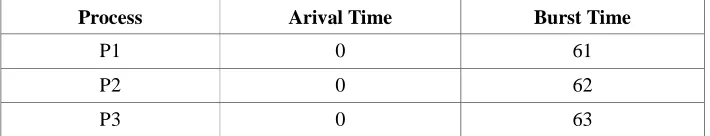
[image:6.612.81.436.613.681.2]

Case 2:Assume four processes arrived at time = 0, with burst time (P1 = 61, P2 = 62, P3 = 63, P4 = 64) as shown in TABLE 3. TABLE 4 shows the comparison between RR and MRR. Figure 5 and Figure 6 shows the gantt chart of RR and MRR.

P1 0 61

P2 0 62

(7)

[image:7.612.31.523.144.429.2]

P4 0 64

RR 20 245 182.5 15

MRR 25,25,25 230 167.5 11

TQ = 20

P1 P2 P3 P4 P1 P2 P3 P4 P1 P2 P3 P4 P1 P2 P3 P4

0 20 40 60 80 100 120 140 160 180 200 220 240 241 243 246 250

Figure 5. Gantt chart of RR

TQ = 25 TQ = 25 TQ = 25

P1 P2 P3 P4 P1 P2 P3 P4 P1 P2 P3 P4

0 25 50 75 100 125 150 175 200 211 223 236 250

Figure 6.Gantt chart of MRR

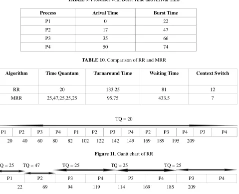
Case 3:Assume four processes arrived at time = 0, with burst time (P1 = 20, P2 = 40, P3 = 80, P4 = 160) as shown in TABLE 5. TABLE 6 shows the comparison between RR and MRR. Figure 7 and Figure 8 shows the gantt chart of RR and MRR.

P1 0 20

P2 0 40

P3 0 80

[image:7.612.44.518.494.674.2]

P4 0 160

RR 20 155 80 13

(8)

TQ = 20

P1 P2 P3 P4 P2 P3 P4 P3 P4 P3 P4 P4 P4 P4 P4

[image:8.612.39.517.113.271.2]

0 20 40 60 80 100 120 140 160 180 200 220 240 260 280 300

TQ = 140 TQ = 25

P1 P2 P3 P4 P4

0 20 60 140 280 300

Figure 8. Gantt chart of MRR

[image:8.612.81.438.350.435.2]

Case 4:Assume four processes arrived at time (P1 = 0, P2 = 2, P3 = 15, P4 = 23), with burst time (P1 = 5, P2 = 25, P3 = 55, P4 = 75) as shown in TABLE 7. TABLE 8 shows the comparison between RR and MRR. Figure 9 and Figure 10 shows the gantt chart of RR and MRR.

TABLE 7. Processes with Burst Time and Arrival Time

P1 0 5

P2 2 25

P3 15 55

[image:8.612.31.517.433.673.2]

P4 23 75

RR 20 80 40 9

MRR 25,25,25,25,25 72.5 32.5 7

TQ = 20

P1 P2 P3 P4 P2 P3 P4 P3 P4 P4

0 5 25 45 65 70 90 110 125 145 160

Figure 9.Gantt chart of RR

TQ = 25 TQ = 25 TQ = 25 TQ = 25 TQ = 25

(9)

0 5 30 55 80 105 130 135 160

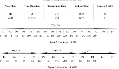
[image:9.612.40.519.201.589.2]

Case 5:Assume four processes arrived at time (P1=0, P2=17, P3= 35, P4=50), with burst time (P1 = 22, P2 = 47, P3 = 66, P4 = 74) as shown in TABLE 9. TABLE 10 shows the comparison between RR an MRR. Figure11 and Figure 12 show the gantt chart of RR and MRR.

TABLE 9. Processes with Burst Time and Arrival Time

P1 0 22

P2 17 47

P3 35 66

P4 50 74

RR 20 133.25 81 12

MRR 25,47,25,25,25 95.75 433.5 7

TQ = 20

P1 P2 P3 P4 P1 P2 P3 P4 P2 P3 P4 P3 P4

0 20 40 60 80 82 102 122 142 149 169 189 195 209

TQ = 25 TQ = 47 TQ = 25 TQ = 25 TQ = 25

P1 P2 P3 P4 P3 P4 P3 P4

0 22 69 94 119 114 169 185 209

REFERENCES

[1] R. J. Matarneh,“Seif-Adjustment Time Quantum in Round Robin Algorithm Depending on Burst Time of the Now Running Proceses”, American Journal of Applied Sciences 6 (10), pp.1831-1837, 2009.

(10)

[3] S. M. Mostafa, S. Z. Rida and S. H. Hamad, “Finding Time Quantum of Round Robin CPU Scheduling Algorithm in General Computing Systems using Integer Programming”, IJRRAS 5(1), pp.64-71, October 2010.

[4] A. Silberschatz, P. B. Galvin and G. Gagne, “Operating System Principles”, 7th Edn., John Wiley and Sons, 2008.

[5] H. S. Behera, R. Mohanty, and D. Nayak, “A New Proposed Dynamic Quantum with Re-Adjusted Round Robin Scheduling Algorithm and Its Performance Analysis,” vol. 5, no. 5, pp. 10-15, August 2010.

(11)