Discovery of Web User Session Clusters Using
DBSCAN and Leader Clustering Techniques
Zahid Ahmed Ansari
Department of CSE, P.A. College of Engineering, Mangalore, India
Abstract— The explosive growth of World Wide Web (WWW) has necessitated the development of Web personalization systems in order to understand the user preferences to dynamically serve customized content to individual users.To reveal information about user preferences from Web usage data, Web Usage Mining (WUM) techniques are extensively being applied to the Web log data. Clustering techniques are widely used in WUM to capture similar interests and trends among users accessing a Web site. Clustering aims to divide a data set into groups or clusters where inter-cluster similarities are minimized while the intra cluster similarities are maximized. This paper describes the discovery of user session clusters using Leader and DBSCAN clustering techniques. These techniques are implemented and tested against the Web user navigational data. Performance and validity results of each technique are presented and compared.
Keywords— Web Usage Mining, User Session Clustering, Leader Clustering, DBSCAN Clustering, Cluster Validation
I. INTRODUCTION
Web Usage Mining [1] is described as the automatic discovery and analysis of patterns in web logs and associated data collected as a result of user interactions with Web resources on one or more Web sites. The goal of Web usage mining is to capture, model, and analyse the behavioural patterns and profiles of users interacting with a Web site. The discovered patterns are usually represented as collections of URLs that are frequently accessed by groups of users with common interests. Web usage mining has been used in a variety of applications such as i) Web Personalization systems [2], ii) Adaptive Web Sites [3][4], iii) Business Intelligence [5], iv) System Improvement to understand the web traffic behaviour which can be utilized to decide strategies for web caching [6], load balancing and data distribution [7], iv) Fraud detection: detection of unusual accesses to the secured data [8], etc.
Clustering techniques are widely used in WUM to capture similar interests and trends among users accessing a Web site. Clustering aims to divide a data set into groups or clusters where inter-cluster similarities are minimized while the intra cluster similarities are maximized. Details of various clustering techniques can be found in survey articles [9]-[11]. The ultimate goal of clustering is to assign data points to a finite system of k clusters. Union of these clusters is equal to a full dataset with the possible exception of outliers. Clustering groups the data objects based only on the information found in the data which describes the data objects and the relationships between them.
Some of the main categories of the clustering methods are [12]: i) Partitioning methods, that create k partitions of a given data set, each representing a cluster. Typical partitioning methods include k-means, k-medoids etc. In k-means algorithm each cluster is represented by the mean value of the data points in the cluster called centroid of the cluster. On the other hand and in k-medoids algorithm, each cluster is represented by one of the data point located near the center of the cluster called medoid of the cluster. Leader clustering is also a partitioning based clustering techniques which generates the clusters based on an initially specified dissimilarity measure, ii) Hierarchical methods create a hierarchical decomposition of the given set of data objects. A hierarchical method can be classified as being either agglomerative or divisive, based on how the hierarchical decomposition is formed. iii) Density- based methods form the clusters based on the notion of density. They can discover the clusters of arbitrary shapes. These methods continue growing the given cluster as long as the number of objects or data points in the “neighborhood” exceeds some threshold. DBSCAN is a typical density-based method that grows clusters according to a density-based connectivity analysis. iv) Grid-based methods quantize the data object space into a finite number of cells that form a grid structure. All the clustering operations are performed on the grid structure. v) Model-based methods, that discover the best fit between data points given a mathematical model. Mathematical model is usually specified as a probability distribution. Clustering techniques have been widely used for mining web usage patterns from web log data [22]-[26].
II. WEBUSAGEDATA CLUSTERING
A number of clustering algorithms have been used in Web usage mining where the data items are user sessions consisting of sequence of page URLs accessed and interest scores on each URL page based on the characteristics of user behaviour such as time elapsed on a page or the bytes downloaded [2]. In this context, clustering can be used in two ways, either to cluster users or to cluster items. In user-based clustering, users are grouped together based on the similarity of their web page navigational patterns. In item based clustering, items are clustered based on the similarity of the interest scores for these items across all users. Mobasher et. al. [13], [14] have used both user-based clustering as well as item-based clustering in a personalization framework based on Web usage mining.
A typical user-based clustering starts with the matrix representing the user sessions or user profiles and partitions this multi-dimensional space into k groups of profiles that are close to each other based on a measure of distance or similarity among the vectors (such as Euclidean or Manhattan distance). Clusters obtained in this way can represent user segments based on their common navigational behaviour or interest shown in various URL items. In order to determine similarity between a target user and a user segment represented by the user session clusters, the centroid vector corresponding to each cluster is computed which is the representation of that user segment. To make a recommendation for a target user u and target URL item i, a neighbourhood of user segments that have a interest scores for i and whose aggregate profile is most similar to u are selected. This neighbourhood represents the set of user segments of which the target user is most likely to be a member. Given that the aggregate profile of a user segment that contains the average interest scores for each item within the segment, a prediction can be made for item i using k-nearest-neighbor approach [15].
We map the user sessions as vectors of URL references in a n-dimensional space. Let Uu1 ,u2, ,un}be a set of n unique URLs
appearing in the preprocessed log and let Ss1,s2 , ,sm}be a set of m user sessions discovered by preprocessing the web log
data, where each user session siScan be represented as , , , }
2 1 u um
u w w
w
s . Each
i u
w may be either a binary or non-binary
value depending on whether it represents presence and absence of the URL in the session or some other feature of the URL. If
i u
w represents presence of absence of the URL in the session, then each user session is represented as a bit vector where
(1) otherwise 0; ; if ; 1
u s
wui i
Instead of binary weights, feature weights can also be used to represent a user session. These feature weights may be based on frequency of occurrence of a URL reference within the user session, the time a user spends on a particular page or the number of bytes downloaded by the user from a page.
III.LEADERAND DBSCANCLUSTERINGTECHNIQUES
Algorithmic details of Leader and DBSCAN clustering techniques are described below.
A. Leader Clustering Algorithm
The leader clustering algorithm [16],[17] is based on a predefined dissimilarity threshold. Initially, a random data point from the input data set is selected as leader. Subsequently, distance of every other data point with the selected leader is computed. If the distance of a data point is less than the dissimilarity threshold, that data point falls in the cluster with the initial leader. Otherwise, the data point is identified as a new leader. The computation of leaders is continued till all the data points are considered. It should be noted that the result of the clustering depends on the chosen distance threshold. The number of leaders is inversely proportional to the selected threshold.
Given a set of m data points X
xi|i1m
, where each data point is a n-dimensional vector. The Euclidean distance between the ith data point xiXand jth
leader ljL(where Lis a set of leaders) is given by :
j j i i j i j i x th k k l x th k k x n k l n
k xk
Algorithm: Leader Clustering
Input: i) Set of m data points X={x1, …, xm},
ii) α, the dissimilarity threshold.
Output: Set of clusters C = {c1, …, ck},
Steps:
1) C,L,j1 // Initialize the cluster and leader sets
2) ljx1 // Initialize x1as the first leader
3) LLlj
4) cjcjx1 5) CCcj
6) for each xiX where i = 2, … m
7) begin
8) argmin ( , )
,lj L i j j l x d j
9) if d2(xi,lj)then
10) cj cjxi
11) else 12) j = j + 1 13) ljxi
14) LLlj
15) cj cjxi
16) CCcj
Fig. 1 describes the algorithmic details of leader clustering algorithm.
B. DBSCAN Clustering Algorithm
[image:4.612.185.414.140.470.2]DBSCAN (Density-Based Spatial Clustering of Applications with Noise) [18] is a density-based data clustering algorithm because it finds a number of clusters starting from the estimated density distribution of corresponding nodes..
Fig. 1 Leader Clustering Algorithm
Given a set of m data points X
xi|i1m
, where each data point is a n-dimensional vector. The Euclidean distance between the two data points xpXand xqXis given byq q p x th k q k m p x th k p k x n k x n
k xk
q x p x d of dimensions of value the is of dimensions of value the is point data each of dimensions of number the is , where (3) 2 1 ) , ( 2
In this algorithm concept of a cluster is based on the notion of “neighborhood” and “density reachability”. Let the ε-neighborhood of a data point xp , denoted as N(xp)is defined as below:
Algorithm: DBSCAN
Input: i) Set of m data points X={x1, …, xm},
ii) ε (epsilon), the neighborhood distance and
iii) , the minimum number of data points required to form a cluster.
Output: Set of clusters C = {c1, …, ck},
Steps:
1) C = Ø.; i = 0;
2) for each xpX and xp.visitedfalse
3) begin
4) xp.visitedtrue
5) Np = N(xp)using (13) 6) if
(xp)
N then
7) xp.noicetrue 8) else
9) i = i + 1
10) C Cci
11) cicixp
12) for each xqN
13) begin
14) if xq.visited false then
15) xq.visitedtrue
16) Nq = N(xq)
17) if N(xq)then
18) Np NpNq
19) if xqcjj1 jithen
20) cicixq
21) endif 22) endif 23) endif 24) end 25) endif 26) end
Let be the minimum number of points required to form a cluster. A point xq is directly density-reachable from a point xp, if xq is
part of ε-neighborhood of xp and if the number of points in the ε-neighborhood of xp are greater than or equal to as specified in
(4).
cluster a for required points of number minimum the
is ) (
(5) )
(
where
x
p x N
p x N q
[image:5.612.114.457.127.663.2].
Fig. 2 DBSCAN Clustering Algorithm
xq is density-reachable from xp if there is a sequence x1 , … , xn of points with x1 = xp and xn = xq where each xi+ 1 is directly
density-connected. ii) If a data point is density-connected to any data point of the cluster, it is part of the cluster as well. Input to DBSCAN algorithm are i) ε (epsilon) and ii) , the minimum number of points required to form a cluster. The algorithm starts
by randomly selecting a starting data point that has not been visited. If the ε-neighborhood of this data point contains sufficiently many points, a cluster is started. Otherwise, the data point is labeled as noise. Later this point might be found in a sufficiently sized ε-neighborhood of a different data point and hence could become part of a cluster. If a data point is found to be part of a cluster, all the data points in its ε-neighborhood are also part of that cluster and hence added to the cluster. This process continues until the cluster is completely found. Then, a new unvisited point is selected and processed, leading to the discovery of a next cluster or noise. Fig. 2 describes the DBSCAN algorithm.
Although DBSCAN can cluster objects given input parameters such as and η, but it is the responsibility of the user to select these parameter values. Such parameter settings are usually empirically set and difficult to determine, especially for high-dimensional data sets.
IV.EXPERIMENTALRESULTS
In order to discover the clusters that exist in user accesses sessions of a web site, we carried out a number of experiments using various clustering techniques. The Web access logs were taken from the P.A. College of Engineering, Mangalore web site, at URL http://www.pace.edu.in. The site hosts a variety of information, including departments, faculty members, research areas, and course information. The Web access logs covered a period of one month, from February 1, 2011 to February 8, 2011. There were 12744 logged requests in total.
A. Pre-processing the Web Log Data
After performing the cleaning operation the output file contained 12744 entries. Total numbers of unique users identified are 16 and the number of user sessions discovered are 206. Table I depicts the results of cleaning and user identification and user session identification steps of preprocessing. Further details of our preprocessing approaches can be found from our previous work [19].
TABLE I
RESULTS OF CLEANING AND USER SESSION IDENTIFICATION
Items Count
Initial No of Log Entries 12744
Log Entries after Cleaning 11995
No. of site ULRs accessed 116
No of Users Identified 16
[image:6.612.215.387.546.645.2]No. of User Sessions Identified 206
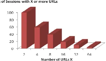
Fig. 3 shows the result of user session identification. It depicts the percentage of user sessions accessing the specified number of URLs.
Fig.3 Percentage of Sessions accessing X No. of URLs
B. User Session Clustering
and C Index which are two quality measures to evaluate the quality of the discovered clusters. These validity measures a described below:
Davies-Bouldin Validity Index: This index attempts to minimize the average distance between each cluster and the one most similar to it. It is defined as [20]:
(6)11 max, ,
1
ki dis ci cj
j c diam i c diam i j k j k DB
An optimal value of the k is the one that minimizes this index.
C Index: It is defined as [21]:
(7) , min max min S S S S C
Here S is the sum of distances over all pairs of objects form the same cluster. Let m be the number of those pairs and Sminis the
sum of the m smallest distances if all pairs of objects are considered. Similarly Smaxis the sum of the m largest distances out of all
pairs. The interval of the C-index values is [0, 1] and this value should be minimized. The results of application of various clustering algorithms are presented in the following subsections.
Leader Algorithm: We conducted the multiple runs of Leader algorithm by selecting the input parameter ε (Dissimilarity Threshold) ranging from ε = 0.5, …, 3.5 in steps of 0.5. For each of these runs we computed the value of the clustering error. We also computed the execution timings, DB index and C index for all of the above runs. Table II describes the results after the application of Leader clustering algorithm.
TABLE II
LEADER CLUSTERING RESULTS
Epsilon (ε)
Error (J)
DB
Index C Index
Execution Time(ms) No. of Clusters 1 1.5 2 2.5 3 3.5 26.19 76.81 216.62 398.81 467.07 624.87 0.3623 0.5061 0.5578 0.7200 0.9084 0.8801 0.0021 0.0348 0.0588 0.0801 0.1878 0.2407 3 2 2 1 2 1 115 86 56 33 26 14
Fig. 4 shows the results of Leader clustering. From the graph it is very clear that the number of discovered clusters is inversely proportional to the dissimilarity threshold ε.
Fig.4 Number of clusters formed Vs. Dissimilarity Threshold ε
We also computed the execution timings, DB index and C index for all of the above runs. Table III describes the results after the application of DBSCAN algorithm for the value of η = 2.
TABLE III
DBSCAN RESULTS
Epsilon (ε)
Error (J)
DB
Index C Index
Execution Time(ms)
No. of Clusters
1
1.5
2
2.5
3
3.5
766.9
805.881
871.2758
881.5672
866.1479
867.23
1.2594
1.3665
0.8415
0.8348
1.0874
0.9092
0.6606
0.1984
0.0766
0.0500
0.0442
0.0463 13
20
24
13
16
17
21
7
2
2
3
3
Fig.5 C Index Vs. Neighbourhood Distance ε
[image:8.612.186.424.121.408.2]The graph plot in Fig. 5 displays the C index as a function of the neighbourhood distance ε, for different values of η (the minimum number of points in a cluster). The graph shows that the C index value improves as we increase the neighbourhood distance ε. It also improves if we decrease the value of η
.
Fig. 6 Number of clusters formed Vs. Neighbourhood Distance ε
The graph plot in Fig. 6 displays the number of clusters formed as a function of the neighbourhood distance ε, for different values of η (the minimum number of points in a cluster). The graph shows that the number of clusters formed decreases as we increase the neighbourhood distance ε. It also decreases if we increase the value of η . The next two graphs compare the results
[image:8.612.195.411.498.625.2]show that in case of Leader clustering, validity index improves for lower values of dissimilarity distance
ε
. In case of DBSCAN, the validity index improves as increase the value of neighbourhood distanceε.
Note that we have set the value of η to 1.Fig. 7 C Index Vs. Epsilon (ε)
The graph plot in Fig.8 displays the Execution Time as a function of Epsilon (
ε
). It is clear from the graph that the Leader algorithm performs much faster than the DBSCAN if we keep the Leader dissimilarity threshold and DBSCAN neighbourhood distance same. Note that we have set the value of η to 1..
Fig. 8 Execution Time in milliseconds Vs. Epsilon (ε)
V. CONCLUSIONS
In this paper we have presented our framework for web usage data clustering for users’ navigational sessions using Leader and DBSCAN clustering algorithms. We provided a detailed overview of these techniques. We also described the mathematical model and algorithm details related to the implementation of these clustering algorithms in order to discover the user sessions clusters. From the results presented in the previous section, we conclude the following points.
A. Although Leader clustering algorithm does not require estimating the value of k at the beginning, it does require estimating the dissimilarity threshold ε.
B. Number of clusters formed in Leader clustering is inversely proportional to the value of dissimilarity threshold ε. C. Leader clustering validity index (C index) improves as we increase the value of the dissimilarity threshold ε. D. DBSCAN algorithm can identify a data point as a noise or outlier.
E. DBSCAN validity index (C index) improves as we decrease the value of the neighborhood distance ε.
F. If we choose the same value for dissimilarity threshold in Leader clustering and neighbor distance in DBSCAN (while keeping η constant), the time performance of Leader clustering much faster than that of DBSCAN.
REFERENCES
[1] J. Srivastava, R. Cooley, M. Deshpande, and P.N. Tan. Web usage mining: Discovery and applications of usage patterns from web data. SIGKDD explorations, 1(2):12–23, 2000.
[2] B. Mobasher. Data mining for web personalization. Lecture Notes in Computer Science, 4321:90, 2007.
[image:9.612.193.406.341.466.2][4] Etzioni O. Perkowitz, M. Adaptive web sites. Communications of ACM, 43:152–158, 2000.
[5] Ajith Abraham. Business intelligence from web usage mining. Journal of Information & Knowledge Management, 2(4):375–390, 2003.
[6] Edith Cohen, Balachander Krishnamurthy, and Jennifer Rexford. Improving end-to-end performance of the web using server volumes and proxy filters. SIGCOMM Comput. Commun. Rev., 28:241–253, October 1998.
[7] Alexandros Nanopoulos, Dimitrios Katsaros, and Yannis Manolopoulos. Exploiting web log mining for web cache enhancement. In WEBKDD 2001 Mining Web Log Data Across All Customers Touch Points, volume 2356 of Lecture Notes in Computer Science, pages 235–241. Springer Berlin / Heidelberg, 2002.
[8] G. Vigna, W. Robertson, Vishal Kher, and R.A. Kemmerer. A stateful intrusion detection system for world-wide web servers. In Computer Security Applications Conference, 2003. Proceedings. 19th Annual, pages 34–43, 2003.
[9] P. Berkhin, “Survey of clustering data mining techniques,” Springer, 2002.
[10] B. Pavel, “A survey of clustering data mining techniques,” in Grouping Multidimensional Data. Springer Berlin Heidelberg, 2006, pp. 25–71. [11] R. Xu and I. Wunsch, D., “Survey of clustering algorithms,” Neural Networks, IEEE Transactions on, vol. 16, no. 3, pp. 645–678, May 2005. [12] M. K. Jiawei Han, Data Mining: Concepts and Techniques. Academic Press, Morgan Kaufmarm Publishers, 2001.
[13] B. Mobasher, H. Dai, T. Luo, and M. Nakagawa. Discovery and evaluation of aggregate usage profiles for web personalization. Data Mining and Knowledge Discovery, 6(1):61–82s, 2002.
[14] Bamshad Mobasher, Robert Cooley, and Jaideep Srivastava. Automatic personalization based on web usage mining. Commun. ACM, 43:142– 151, August 2000.
[15] Jonathan L. Herlocker, Joseph A. Konstan, Al Borchers, and John Riedl. An algorithmic framework for performing collaborative filtering. In Proceedings of the 22nd annual international ACM SIGIR conference on Research and development in information retrieval, SIGIR ’99, pages 230–237, New York, NY, USA, 1999. ACM.
[16] H. Spath, Cluster Analysis * Algorithms for Data Reduction and Classi"cation of Objects Ellis Horwood Limited, West Sussex, UK, 1980. [17] T. R. Babu, M.N. Murty, Comparison ofGenetic algorithmbased prototype selection scheme, Pattern Recognition 34 (2) (2001) 523–525
[18] Martin Ester, Hans-Peter Kriegel, Jörg Sander, Xiaowei Xu (1996-). "A density-based algorithm for discovering clusters in large spatial databases with noise" Proceedings of the Second International Conference on Knowledge Discovery and Data Mining (KDD-96). pp. 226–231.
[19] Zahid Ansari, A. Vinaya Babu, Waseem Ahmed and Mohammad Fazle Azeem, “A Fuzzy Set Theoretic Approach to Discover User Sessions from Web Navigational Data”, in International Conference on IEEE Recent Advances in Intelligent Computational Systems, Trivandrum Sep. 22-24 2011, pp. 879-884.
[20] D.L. Davies, D.W. Bouldin. A cluster separation measure. 1979. IEEE Trans. Pattern Anal. Machine Intell. 1 (4). 224-227.
[21] Hubert, L. and Schultz, J. Quadratic assignment as a general data-analysis strategy. British Journal of Mathematical and Statistical Psychology, 29, 190-241, 1976.
[22] Zahid Ansari , Mohammad Fazle Azeem, A. Vinaya Babu and Waseem Ahmed. “A Fuzzy Clustering Based Approach for Mining Usage Profiles from Web Log Data” International Journal of Computer Science and Information Security, pp. 70-79 Vol. 9, No. 6, June 2011.
[23] Zahid Ansari, Waseem Ahmed , M.F. Azeem and A.Vinaya Babu. “Discovery of Web Usage Profiles Using Various Clustering Techniques”. International Journal of Computer Information Systems, pp. 18-27 Vol. 1, No. 3, July 2011.
[24] Zahid Ansari, A. Vinaya Babu, Waseem Ahmed and Mohammed Fazle Azeem. “A Comparative Study of Mining Web Usage Patterns Using Variants of k-Means Clustering Algorithm”. International Journal of Computer Science and Information Technologies, pp. 1407-1413 Vol. 2 No. 4, July 2011. [25] Zahid Ansari, A.Vinaya Babu, M.F. Azeem and Waseem Ahmed. “Quantitative Evaluation of Performance and Validity Indices for Clustering the Web
Navigational Sessions” World of Computer Science and Information Technology Journal pp. 217-226, Vol. 1, No. 5, June 2011.