Optical Orbit Determination and Propagation of Leo Satellites Applying Variable Step Integrations

5

IX

September 2017

Optical Orbit Determination and Propagation of

Leo Satellites Applying Variable Step Integrations

A.M.Abdelaziz1, I.A.Hassan2, K.I.Khalil3, A.B.Ahmed4 and Y.A.Abdelaziz5 1, 3, 5

National research institute of astronomy and geophysics (NRIAG), Cairo, Egypt

2,4

Astronomy and meteorology department, faculty of science, Al-Azhar University, Cairo, Egypt

Abstract: This paper represents optical orbit determination and propagation of low Earth orbit (LEO) satellites (Iridium 53). Angles only methods which apply on angular measurements from optical sensor provide initial position and velocity of satellites then we can refine our results using least square technique. The actual motion of a satellite is affected by various forces including gravitational and non-gravitational ones. Equations of motion can be solved by integration numerically for all perturbations included Earth's gravitational potential atmospheric drag forces, third body and solar radiation pressure by using Runge Kutta -Fehlberg method and Shampine-Gordon method these methods were treated by Cowell’s technique.

Keywords: Orbit determination-orbit propagation- low earth satellites- numerical integration –variable step integration. I. INTRODUCTION

Satellite Orbit Determination (OD) can be described as the method of estimate the position and velocity (i.e., the state vector, state, or ephemeris) of an Earth-orbiting satellite. In this paper, determine the best estimate of the satellite's state at some epoch from angles only observation applying statistical estimation techniques (least square technique) that account for the dynamical environment in which the motion occurs for Iridium 53 satellite which it’s altitude about 780 km with eccentricity 0.000198. We design an orbit propagation model using the Cowell's method which gives the ephemeris of the artificial satellite at any given time. The perturbations important for the orbits of low earth satellites are the Earth's gravitational potential, atmospheric drag, the gravitational influences of the sun and moon, and the solar radiation pressure. For precise orbit propagation in Cowell' method, 360 x 360 spherical harmonic coefficients can be applied and the JPL DE405 ephemeris files were used to generate the range from earth to sun and moon. Runge-Kutta single step method and Shampine-Gordon multi step method with variable step-size control is used to integrate the orbit propagation equations.

II. ORBIT DETERMINATION

A. Initial orbit determination

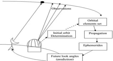
Initial orbit determination is the process of collecting a set of measurements and calculating the position and velocity of a satellite at a particular time or determining a set of six orbital elements that define the size, shape, and orientation of the orbit of the object. Figure (1) show the orbit determination process.

To derive six orbital elements, the same numbers of independent observational values are required, so three observations must be available. For this paper, the Gauss method, the Double R iteration method, and the Gooding method will all be used. Both the Gibbs and Herrick-Gibbs methods will be used to refine the velocity estimate found by the Gauss method.

Figure (1): representation of orbit determination.

B. Least square

We used a weighted least-squares estimator to refine the orbit derived from the IOD method. The batch-least squares process is limited in the number of states estimated. These include position, velocity, solar-radiation pressure correction, ballistic coefficient correction, and measurement biases. The primary function is to refine the IOD estimate (or other initial estimate) sufficiently using a more complete force model [3].

III. ORBIT PROPAGATION The equations of perturbed motion of a satellite is written as

3 p

r

r

a

r

µ

 



v

_v

_v

&

&

Where r is the position vector of the satellite measured from the center of the primary body, µ is the gravitational constant and ap is the sum of all the perturbing accelerations. The equations of motion is solved by numerical integration. The perturbations that effects the satellite can be classified into two types:

Gravitational perturbation: such as; Earth's gravitational, the gravitational influences of the sun and moon. Non-gravitational perturbation: such as; Atmospheric Drag, Solar Radiation Pressure.

A. Acceleration due to Geopotential

The gravitational potential due to the Earth can be expressed in terms of a series of spherical harmonic functions. In a body fixed reference coordinates system as,





, , ,

2 0

( , , )

(

)

[sin( )]

cos(

)

sin(

)

n n

E

n m n m n m

n m

R

U r

P

C

m

S

m

r

r

r





 











_{ }



φ = the geocentric latitude of the satellite.

λ = the geocentric east longitude of the satellite.

r = the geocentric distance of the satellite,

: r = │r│= + + ,

sin ( )

z

r





arctan(

y

)

x





RE = Radius of the Earth.

Pn,m= associated Legendre polynomials of degree n and order m. Cn,m, Sn,m = the gravitational coefficients.

The acceleration due to the Earth’s gravity field can be obtained by finding the partial derivative or gradient of the potential function[3]

( , )

g

B. Acceleration due to drag

The Atmospheric drag is the most complex and the most difficult force acting on low earth orbits. The basic equation for atmospheric drag combines several factors; I'm showing it here as a specific force or acceleration:

2

1

2

C A

V

a

v

m



V

 

v

v

v

Where (ρ) Atmospheric density (kg/m3), (Cd) is the drag coefficient appropriately equal 2.2 for a sphere or rotating cylinder, (A) is the effective cross- sectional area of the body, (m) is the satellite mass and (v) is the satellite atmosphere relative speed[].

C. Acceleration due to the third body

The Sun and the Moon, have a greater effect on satellites in higher altitude orbits. Their effects become noticeable about when the effects of drag begin to diminish. Because the cause of perturbations from Sun and Moon is the gravitational attraction, which is conservative, it's reasonable to use a disturbing-function solution [2]. The basic equation for acceleration contribution of the moon represented by a point mass is given by

3 3

M sat E M

moon M

M sat E M

r

r

a

r

r







 

_



_





v

v

v

μM= gravitational constant of the moon.

rM-sat= position vector from the moon to the satellite rE-M= position vector from the earth to the moon.

Similarly, the acceleration contribution of the sun represented by a point mass is given by

3 3

s sat E s

sun M

s sat E s

r

r

a

r

r







 

_



_





v

v

v

D. Acceleration due to solar radiation pressure

The particle radiation, continuously emitted by the Sun, has two effects on a satellite. These are the direct radiation pressure, resulting from the interaction of the solar radiation with the satellite, and the indirect, Earth-reflected portion (albedo).

The influence of this force depends on altitude and the solar activity. It is very important to quantify the effect of solar radiation pressure during periods of intense solar storms as it can dominate all other perturbation forces, especially at higher altitudes[]. The acceleration due to solar radiation pressure depends on the mass and surface area of the satellite and is defined by

sr r su st

srp

su st

P C A

r

a

m

r





 

v

v

v

Where

Psr = solar pressure

Cr = radiation pressure reflectivity coefficient Asu = area exposed to the Sun's radiation

rsu-st = position vector from the sun to the satellite

E. Numerical Integration Methods

Numerical integration methods can be divided into several categories. Two main categories are single-step and multi-step, and refer to the number of steps used when integrating to the next point. Single-step techniques combine the state at the epoch time with the rates from several other times to calculate the update. Multi-step techniques, also called predictor-corrector algorithms, calculate an initial estimate based on previous estimates of the rate of change (predictor) and then use the estimated value to further refine the result (corrector). Multi-step techniques are generally faster than single-step techniques, although they suffer some drawbacks, including the need for a start-up routine because they require back values.

integration methods change the step size at each step to meet some tolerance for the local error. The local error is estimated at each step, and the step size is adjusted so that the estimated error at the next step will be approximately equal to the tolerance. The local error estimate is made by comparing two integrations made of different orders. For instance, the Runge-Kutta-Fehlberg method estimates the local error by comparing the result of fourth-order and fifth-order Runge-Kutta formulas. For multi-step integrators, local error estimates can be made by using predictor and corrector formulas of a different order.

Numerical integration techniques can also be classified according to the type of formulation. Single-integration techniques calculate the velocity given the acceleration, and then the position given the velocity. Double-integration techniques calculate the position directly from the acceleration [Berry 2004].We will use the Runge-Kutta Fehlberg method and Shampine-Gordon method for numerical integration. Both methods are variable step size but the first method is single step while second is a multi-step method [4].

IV. NUMERICAL RESULTS

Table (1) show the results of orbit determination for Iridium 53 satellite which observed from a station at 44N,76.5W, H = 79 m, on January 06,2016 by Celestron NexStar 11-inch attached with SBIG ST-9 Dual CCD Camera [1].

Table (1): The results and comparison between angles only orbit determination method.

In this section we shows and discuss the effect of perpetuation forces on the keplerian orbital elements of Iridium53 satellite which results from orbit determination section. The equation of motion with the existence of individual perturbation and the effect of all perturbation is solved by using Runge-Kutta method and Shampine-Gordon method these methods were treated by Cowell’s technique.

Figures (2-7) show the comparison between Runge-Kutta method (blue line) and Shampine-Gordon (red line). From our numerical results and these figures it can be seen that the Shampine-Gordon method is more accurate than Runge-Kutta method but take much time.

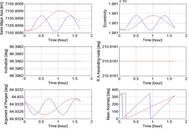
In case of j2 only and according to Figure (3), the perturbation in the semi major axis of the orbit has a periodic behavior. It changes about 18 km during one revolution. Also, the inclination of the orbit changes of about 0.0046 degree in one revolution. Eccentricity has a complex behavior it seems to have two types of periodic variations. Its maximum change is about 0.0017.The right ascension

TLE Gauss-Gibbs

(diff)

Gauss-H.Gibbs

(diff)

Double R iteration

(diff)

Gooding

(diff)

a

(km) 7155.8056

7155.5828 (0.2228) 7155.6689 (0.1367) 7155.01885 (0.7867) 7155.12094 (0. 68466)

e 0.0001

0.0022 (-0.0021) 0.0295 (-0.0294) 0.8021 (-0.802) 0.0009 (-0.0008)

I (°) 86.3962 86.4904

(-0.0942) 86.4662 (-0.07) 89.1500 (-2.7) 86.4573 (-0.0611)

Ω (°) 210.8161

210.5829 (0.2332) 210.5962 (0.2199) 209.0888 (1.7273) 210.6005 (0.2156)

ω (°) 84.9325

255.7077 (-170.7) 62.1965 (22.7) 1.1345 (83.7) 203.4774 (-118.5)

n(rev /day) 14.342186

of ascending node has a secular behavior as well as a periodic change with low amplitude. It changes about 0.0287 degree during one revolution. Argument of Perigee has a periodic variation as well as a simple secular. Mean anomaly of the satellite has periodic variations.

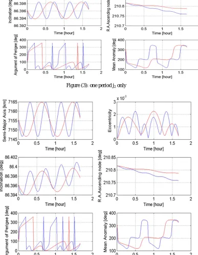
Figure (4) show the behavior of keplerian element due to the geopotential perturbation up to degree and order 16. That is the same behavior such as occurred in j2 case with slightly change.

Figure (5) shows the perturbations due to the air drag force using NRLMSISE00 atmosphere model. The effect on the semi major axis of the orbit is about 0.063 m in one revolution secular. Also, the inclination and the right ascension of ascending node have variation about 10-7 secularly. Eccentricity has periodic variation about 10-7, argument of Perigee has a periodic variation about 5×10-4 degree as well as a secular and mean anomaly has periodic variation.

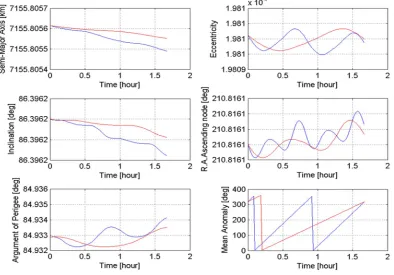
Figure (6) shows the perturbations due to the third body effect on orbit. The variations of the semi major axis are periodic and is about 1.1 meter in one revolution, the inclination has the secular variation about 10-4 degree. The eccentricity has a periodic variation about 2×10-7 also, the right ascension of ascending node behavior is periodic. The argument of perigee has also periodic behavior and maximum change of about 0.08 degree can be seen in one revolution and the mean anomaly has a periodic variations as well.

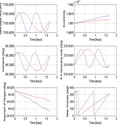
Figure (7) show the variations on the elements due to the solar radiation pressure. The semi major axis of the orbit, inclination, right ascension of ascending node, and the mean anomaly of the satellites have periodic behavior about 0.1 meter for semi major axis and 10-5 for inclination and right ascension of ascending node , whereas the argument of perigee and eccentricity variations are secular about 4×10-8 and 0.01 degree respectively.

The summary of the above numerical results are presented in table (5.4) which show that the maximum values of the perturbations in orbital elements due to each one of the disruptive accelerations. The word complex means a combination of secular and periodic variations.

As one can see from the table, the geopotential acceleration has the largest effect .The semi major axis of the orbit has periodic variations under almost all of the perturbing accelerations except the air drag. The inclination’s behavior is secular for the air drag and the third body effect, and for the rest of the acceleration it is periodic. The eccentricity behaves periodically for geopotential, the third body and air drag. The right ascension of the ascending node acts periodically for solar radiation, but it acts as secular for the rest of the accelerations. The argument of perigee has just secular variation due to the solar radiation. The mean anomaly usually varies periodically.

Figure (3): one period j2 only

Figure (5): one period drag

Figure (7): one period solar radiation pressure

Table (5.4). Perturbing accelerations and orbital elements during one period

a (m) e I(deg) Ω(deg) ω(deg) M

geopotential 18351

Periodic

0.001712 Periodic

0.0046 Periodic

0.0287

secular Complex Periodic

Air drag 0.063

Secular

10-7 periodic

10-7 Secular

10-7 Secular

5×10-4

Complex Periodic

Third body 1.1

Periodic

2×10-7 periodic

10-4 Secular

10-7 periodic

0.08

periodic Periodic

Solar radiation 0.1

Periodic

4×10-8 Secular

10-5 periodic

10-5 periodic

0.01

V. CONCLUSION

In this paper, the mathematical models were designed to orbit determination and propagation for Iridium 53 satellite which it’s altitude about 780 km with eccentricity 0.000198 from observation using angles only methods for initial orbit determination, a least square method for refining orbit and high precision orbit propagation in Cowell form. The results were as the following form:

A. The methods of angels only observation tested in this thesis were the Gauss method (supplement with Gibbs and Herrick-Gibbs method), the Double R method, and the Gooding method. The Gauss method performs remarkably well when the data is separated 10º or less, and if the vectors are too close to one another we must use Herrick-Gibbs method Other than we can use Gibbs method.

B. The Double R method being poorly defined when the first and third observation are close together.

C. The Gooding method is the best method to estimate the orbit.

D. The geopotential acceleration has the largest effect. The semi-major axis of the orbit has periodic variations under almost all of the perturbing accelerations except the air drag. The inclination’s behavior is secular for the air drag and the third body effect, and for the rest of the acceleration, it is periodic. The eccentricity behaves periodically for geopotential, the third body, and air drag. The right ascension of the ascending node acts periodically for solar radiation, but it acts as secular for the rest of the accelerations. The argument of perigee has just secular variation due to the solar radiation. The mean anomaly usually varies periodically.

REFERENCES

[1] A.M.Abdelaziz, I.A.Hassan, K.I.Khalil and A.B.Ahmed, “Initial orbit determination from angles only observation for low earth orbit”,paper conference, the 9 th International Conference for Basic Sciences 27 – 29 March, 2017, Cairo, Egypt 2017.

[2] Montenbruck, O. and Gill, E. Satellite Orbits - Models, Methods, and Applications. Springer-Verlag, Heidelberg, 2000. [3] Vallado, David A. Fundamentals of Astrodynamics and Applications. New York, NY: McGraw-Hill, 2013.

[4] Berry, Matthew M. A, “Variable-step Double-integration Multi-step Integrator”. Ph.D. Dissertation. Virginia Polytechnic Institute and State University, 2004.

a (m) e I(deg) Ω(deg) ω(deg) M

geopotential 18351 Periodic 0.001712 Periodic 0.0046 Periodic 0.0287 secular

Complex Periodic