for Complex-Valued Hopfield Associative
Memory
Naoki Masuyama(B)and Chu Kiong Loo
Faculty of Computer Science and Information Technology, University of Malaya, 50603 Kuala Lumpur, Malaysia
[email protected],[email protected]
Abstract. This paper discusses a complex-valued Hopfield associative memory with an iterative incremental learning algorithm. The mathe-matical proofs derive that the weight matrix is approximated as a weight matrix by the complex-valued pseudo inverse algorithm. Furthermore, the minimum number of iterations for the learning sequence is defined with maintaining the network stability. From the result of simulation experiment in terms of memory capacity and noise tolerance, the pro-posed model has the superior ability than the model with a complex-valued pseudo inverse learning algorithm.
Keywords: Associative memory
·
Complex-valued model·
Incremental learning1
Introduction
In the past decades, numerous types of “Artificial Intelligence” models have been proposed in the field of computer science in order to realize the human-like abilities based on the analysis and modeling of essential functions of a bio-logical neuron and its complicated networks in a computer. It has been noted that one of the interesting and challenging subjects is the imitation of memory function of the human brain. In the past decades, several types of artificial asso-ciative memory models and its improvements have introduced such as Hopfield Associative Memory (HAM) [7], and Bi-/Multi-directional Associative Memory (BAM, MAM) [6,11]. However, the majority of models are limited as offline and one-shot learning rules. Storkey and Valabregue [14] proposed an incremental learning algorithm for HAM based on the Hebb/Anti-Hebb learning. Chartier and Boukadoum [3] also proposed and analyzed the model with a self-convergent iterative learning rule based on the Hebb/anti-Hebb approach, and a nonlinear output function Diederich and Opper [4] proposed a Widrow-Hoff type learn-ing. However, the convergence of these models is quite slow when the memory patterns are correlated. The local iterative learning, on the other hand, which is proposed by Blatt and Vergini [2] can be dealt with above kind of problems.
c
Springer International Publishing AG 2016
Moreover, this model is able to define the minimum number of learning iterations with maintaining a network stability.
In regard as events in the real world, information representation using binary or bipolar state is insufficient. Jankowski et al. [9] have introduced complex-valued Hopfield Associative Memory (CHAM) with neurons processing a complex-valued discrete activation function. Conventionally, numerous studies that improve complex-valued models are introduced based on the improvements for real-valued models. Lee [13] applied a complex-valued projection matrix to CHAM (PInvCHAM) and analyzed the stability of the model by using energy function. The learning algorithm of these models, however, are characterized by a batch learning. Isokawa et al. [8] analyzed the stability of complex-valued Hopfield model with from a local iterative learning scheme viewpoint though the learning algorithm is Hebb learning base. In this paper, we introduce a local iterative incremental learning with CHAM based on Blatt and Vergini learning algorithm [2]. Here, we shall call the proposed model as BVCHAM. The note-worthy features of BVCHAM are described as follows; (i) the resultant of weight matrix in BVCHAM is approximated to the projection matrix operation. The network is able to store the patterns though the number of stored patternspis larger than the number of neuronsN (It is known that the memory capacity is limited asp < N with a projection matrix learning model.), and (ii) the learning algorithm is guaranteed to calculate a weight matrix within a finite number of iterations with keeping a network stability.
The paper is divided as follows; Sect.2describes the dynamics of BVCHAM. Section3 presents the network stability analysis for BVCHAM. In Sect.4, it will be presented simulation experiments of BVCHAM in terms of the memory capacity and noise tolerance comparing with PinvCHAM. Concluding remarks are presented in Sect.5.
2
Dynamics of a Local Iterative Learning for CHAM
This section presents the dynamics of a proposed model, we shall call as BVCHAM.
Let us suppose that the model stores complex-valued fundamental memory vectors Xp, where Xp = [xp
1, xp2, . . . , xpN]T, N denotes the number of neurons, andpdenotes the number of patterns. The componentsxpi are defined as follows;
xpi ∈exp [j2πn/q]q−
1
n=0, i= 1,2, . . . , N (1)
whereq denotes a quantization value on the complex valued unit circle. Here, supposing a new pattern Xl stores to the network by updating the weight matrix W(l−1) that already has (l−1) patterns embedded. X(l) is
pre-sentednl times to the network as follows;
W(l)=W(l−1)+ nl
d=1
where, ΔW is defined as a following;
ΔWd(l)=kd−1xli−hi xlj−hj
/N. (3)
The local fieldhi which changes (d−1) times is performed as a following;
hi= N
j=1
Wij(l−1)+ d−1
r=1
Wr(l)
ij
xlj. (4)
Similar with Eq. (4), the local fieldhj is defined. Here, the minimum number of iterationsnlcan be defined as a following;
nl≥logk N/(π/q−T)
2
(5) where, a parameter k, called memory coefficient, is a real number that belongs to the interval 0 < k ≤4, and a parameter T is set between 0≤ T < π/q. It allows to perform in order to achieve aligned local fields with values of at leastT
[2].qdenotes a quantization value on the complex unit circle, which is described in a following part. The iterative weight update is performed until satisfying the criterion as T >error, namely;
T > = N i=1 arg hi Xl i . (6)
In summary, the process of weight update is described as Algorithm1. For the association process, the self-connections eliminated weight matrixW is utilized. On the other hand, the weight matrixW which is calculated by Algorithm1 is applied to the further incremental learning process.
Algorithm 1. An algorithm for a weight matrixW(l)
Require: weight matrixW(l−1), fundamental memory vectorXl, error parameterT, memory coef-ficientk
Ensure: weight matrixW(l) if l= 1then
InitializeW as a zero matrix
end if
Setd= 1
Calculate an errorusing Eq. (6)
whiled≥nland > Tdo
Calculate a weight matrixW(l)using Eqs. (2) and (3) Calculate an errorusing Eq. (6)
Setd←d+ 1
end while
The activation function is a complex projection function that operates on each component of the state vector as a following;
φ(Z) =
⎧ ⎪ ⎨ ⎪ ⎩
exp(j2πn/q), If arg
Z
exp(j2πn/q)
< π/qandZ = 0
previous state, IfZ = 0
where, arg(α) denotes the phase angle ofαwhich is taken to range over (−π, π).
q denotes a quantization value on the complex unit circle, n takes an integer. We utilized a discrete complex unit circle model to determine recalled signals.
Thus, the dynamics of network is summarized as follows;
⎧ ⎨ ⎩
h(t)=W
X(t) (8)
X(t+1)=φ
h(t)
(9)
The stationary conditions for the recalled memory vector are described as a following;
0≤arg
h Xp
<π
q. (10)
3
Network Stability Analysis
In this section, based on Blatt and Vergini algorithm [2], the conditions of net-work stability in BVCHAM will be discussed, and it will be derived a criterion for the number of iterationsnlto guarantee the stability ofXl. Here, Dirac nota-tion inCN is utilized for simplifying the representation of proofs. Thus, Eqs. (3) and (4) can be described as follows;
ΔWdl=
kd−1 N |X
l−hXl−h| (11)
|h=
W(l−1)+ d−1
r=1 ΔWrl
|Xl (12)
here, it satisfies|Xl−h†=Xl−h|.
First of all, the changes of weight connection when a new memory vector is repeated to the network is analyzed. Here,ΔWd(l)(1≤d) is defined as a following;
d
r=1
ΔWr(l)=Q
(l)
d
E(l−1)|XlXl|E(l−1)
N (13)
where,
E(l)=I−W(l) (14)
here,Idenotes an identity matrix which has same dimension with W(l). It assumes that Eq. (13) holds ford-th iteration in order to prove (d+ 1)-th iteration. The difference of weight connection between the d-th and (d+ 1)-th iteration with a memory vectorXland its local fieldhis expressed by Eqs. (12), (13) and (14), as follows;
|Xl−h= (1−a(l)
where,
a(l)= X
l|E(l−1)|Xl
N . (16)
The change in (d+ 1)-th iteration is expressed by Eqs. (11) and (15) as a following;
ΔWd(+1l) =kd
1−a(l)Q(dl)
2E(l−1)|XlXl|E(l−1)
N . (17)
Comparing with Eqs. (13) and (17), it can be regarded as a proportional relation with the same operator. Thus, the following recurrence relations are obtained;
Q(1l)= 1 (18)
Q(dl)=Q(d−l)1+kd− 11−
a(l)Q(d−l)1
2
. (19)
From the Eqs. (13) and (14), Eq. (2) is represented as a following;
E(l)=E(l−1)−Q(nll)
E(l−1)|XlXl|E(l−1)
N . (20)
Therefore, when a new memory vector is presented to the network, an opera-tor which is proportional to the projecopera-tor ontoE(l−1)|Xlis added to the weight connection. According to Eq. (11),ΔWincreases exponentially with the number of iterations d. However, if the following condition is satisfied, the elements of
ΔW remain finite, i.e.;
0≤ φ|E(l)|φ ≤ φ|φfor all|φ ∈CN. (21)
In the first learning step, it maintainsE(0) =I and Q(1)d = 1. Furthermore, based on Cauchy–Schwarz inequality, Eq. (21) is verified forl= 1. Here, assum-ing that Eq. (21) is valid for l. Then, the eigenvalues ofE(l) take between 0 to 1. Therefore, the following condition is satisfied;
E(l)|φ2≤ φ|E(l)|φ. (22)
Let us suppose that a(l+1) = 0, E(l)|Xl+1 = 0 is derived from Eqs. (16)
and (22), thenE(l+1)=E(l) is maintained from Eq. (20). Thus, Eq. (21) is also
satisfied for (l+1). In contrast, in case ofa(l+1)= 0, it is proved by the inductive
hypothesis 0 < a(l+1) ≤ 1. Furthermore, according to [2], following conditions
are maintained;
0< a(l)Q(dl)≤1. (23)
1−a(l)Q(dl)≤
k−d a(l)
. (24)
distance between|Xμand|hdecreases exponentially with the number of itera-tions. This is derived by the induction process. First of all, the following condition is maintained by the Eqs. (14) and (22);
|Xμ −W(l)|Xμ2≤ Xμ|E(l)|Xμ. (25)
Here, Eq. (20) is generalized as a following;
E(l)=E(μ)−
l
ν=μ+1 Qνnν
E(ν−1)|XνXν|E(ν−1)
N . (26)
Then,Xμ|multiplied on the left hand side, and|Xμmultiplied on the right hand side to Eq. (26), therefore;
Xμ|E(l)|Xμ ≤ Xμ|E(μ)|Xμ. (27)
For the Eq. (20) with a μ-th memory vector,Xμ| is multiplied on the left hand side, and|Xμis multiplied on the right hand side, i.e.;
Xμ|E(μ)|Xμ=Xμ|E(μ−1)|Xμ −Q(μ)
nμ
(Xμ|E(μ−1)|Xμ)2
N . (28)
Considering with Eq. (16), Eq. (28) is described as a following;
Xμ|E(μ)|Xμ=N a(μ)1−
a(μ)Q(nμμ)
. (29)
Furthermore,N anda(μ) multiplied to Eq. (24) with a μ-th memory vector,
i.e.;
N a(μ)
1−a(μ)Q(nμμ)
≤N k−nμ. (30)
From Eqs. (25), (27), (29) and (30), the following condition is obtained;
|Xμ −W(l)|Xμ2≤ Xμ|E(l)|Xμ ≤ Xμ|E(μ)|Xμ
=N a(μ)
1−a(μ)Q(nμμ)
≤N k−nμ. (31)
According to the stability condition as Eq. (10), Eq. (31) is described as a following;
|Xμ −W(l)|Xμ2≤N k−nμ ≤
π q −T
2
(32)
4
Simulation Experiment
This section presents the simulation experiments comparing with a pseudo inverse learning model (PInvCHAM) [1] and a proposed model (BVCHAM), in terms of memory capacity and noise tolerance.
4.1 Condition
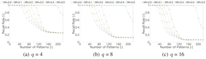
Table1 shows the simulation conditions to evaluate the memory capacity and the noise tolerance. In this experiment, the number of pairspis increased from 1 to 220 at intervals of 10 (p= 1,10,20, . . . ,220). Noise tolerance is a significant property for the associative memory. Typically, “noise” is roughly divided into two types in associative memory. One is the similarity of the stored patterns, another is the stored patterns contain noise itself. Due to the proposed model has the similar properties with a pseudo inverse learning model, it is expected that the proposed model is able to learn the correlated memory vectors without errors. In this paper, therefore, we consider about a latter type of noise which is contained in an initial input with 0 to 50 [%] by the salt & pepper noise. Furthermore, it is known that the ability of a complex-valued associative memory is dependent upon the number of divisions of a complex-valued unit circle. Here, we set 4, 8 and 16 divisions for this simulation.
Table 1.Simulation condition.
Number of pairsp : 1–220 Number of neuronsN: 200
Number of divisionsq: 4, 8, 16
Data set configuration: Amplitude: 1.0, Phase: Rand
4.2 Result
In Fig.1, PInvCHAM maintains the high recall rate, especiallyN R= 0.0. How-ever, due to the limitation of the pseudo inverse learning, the recall rate is suddenly dropped under the condition N ≤ p. As shown in Fig.2, due to the weight matrix of BVCHAM can be approximated as the weight matrix by a pseudo inverse learning, the recall rate of BVCHAM shows the similar or supe-rior results (especially in Fig.2(a)) than PInvCHAM. Here, it focuses on the results with N R = 0.0 in Fig.2. Since the weight matrix of BVCHAM is not equal to the identity matrix at p=N, BVCHAM is able to maintain the high recall rate than PInvCHAM even if the condition is under N≤p.
(a)q= 4 (b)q= 8 (c)q= 16
Fig. 1.Results of recall ratio for a pseudo inverse learning model.
(a)q= 4 (b)q= 8 (c)q= 16
Fig. 2.Results of recall ratio for a BV incremental learning model.
5
Conclusion
This paper introduced a local iterative incremental learning algorithm for a complex-valued Hopfield associative memory. Furthermore, we presented the net-work stability analysis which derived the weight matrix of BVCHAM is approx-imated as a weight matrix from a complex-valued pseudo inverse learning algo-rithm, and the minimum number of iterations with maintaining a network con-vergence. From the result of simulation experiment in terms of memory capacity and noise tolerance, BVCHAM has the superior ability than the models with the Hebb learning and a complex-valued pseudo inverse learning algorithm. Note-worthy, unlike the model with a pseudo inverse learning algorithm, the proposed model is able to maintain the high recall rate even if the number of stored pat-terns is larger than the number of neurons.
As a future work, we will extend the proposed incremental learning algorithm to hetero-association models, such as bi/multi-directional associative memory models [10].
[image:8.439.43.381.182.279.2]References
1. Albert, A.: Regression and the Moore-Penrose Inverse. Academic Press, New York (1972)
2. Blatt, M.G., Vergini, E.G.: Neural networks: a local learning prescription for arbi-trary correlated patterns. Phys. Rev. Lett.66(13), 1793 (1991)
3. Chartier, S., Boukadoum, M.: A bidirectional heteroassociative memory for binary and grey-level patterns. IEEE Trans. Neural Netw.17(2), 385–396 (2006) 4. Diederich, S., Opper, M.: Learning of correlated patterns in spin-glass networks by
local learning rules. Phys. Rev. Lett.58(9), 949 (1987)
5. Gardner, E.: Optimal basins of attraction in randomly sparse neural network mod-els. J. Phys. A: Math. Gen.22(12), 1969 (1989)
6. Hagiwara, M.: Multidirectional associative memory. In: International Joint Con-ference on Neural Networks, vol. 1, pp. 3–6 (1990)
7. Hopfield, J.J.: Neural networks and physical systems with emergent collective com-putational abilities. Proc. Nat. Acad. Sci.79(8), 2554–2558 (1982)
8. Isokawa, T., Nishimura, H., Matsui, N.: An iterative learning scheme for multistate complex-valued and quaternionic Hopfield neural networks (2009)
9. Jankowski, S., Lozowski, A., Zurada, J.: Complex-valued multistate neural asso-ciative memory. IEEE Trans. Neural Netw.7(6), 1491–1496 (1996)
10. Kobayashi, M., Yamazaki, H.: Complex-valued multidirectional associative mem-ory. Electr. Eng. Jpn.159(1), 39–45 (2007)
11. Kosko, B.: Constructing an associative memory. Byte12(10), 137–144 (1987) 12. Krauth, W., M´ezard, M.: Learning algorithms with optimal stability in neural
networks. J. Phys. A: Math. Gen.20(11), L745 (1987)
13. Lee, D.L.: Improvements of complex-valued Hopfield associative memory by using generalized projection rules. IEEE Trans. Neural Netw.17(5), 1341–1347 (2006) 14. Storkey, A.J., Valabregue, R.: The basins of attraction of a new Hopfield learning