Stochastic Process Optimization Technique

http://dx.doi.org/10.4236/am.2014.519293

Stochastic Process Optimization Technique

Hiroaki Yoshida

1

_{, Katsuhito Yamaguchi}

2

_{, Yoshio Ishikawa}

1

1_{College of Science and Technology, Nihon University, Chiba, Japan} 2_{Junior College, Nihon University, Chiba, Japan}

Email: [email protected]

Received 9 September 2014; revised 29 September 2014; accepted 10 October 2014

Copyright © 2014 by authors and Scientific Research Publishing Inc.

This work is licensed under the Creative Commons Attribution International License (CC BY). http://creativecommons.org/licenses/by/4.0/

Abstract

The conventional optimization methods were generally based on a deterministic approach, since their purpose is to find out an accurate solution. However, when the solution space is extremely narrowed as a result of setting many inequality constraints, an ingenious scheme based on expe-rience may be needed. Similarly, parameters must be adjusted with solution search algorithms when nonlinearity of the problem is strong, because the risk of falling into local solution is high. Thus, we here propose a new method in which the optimization problem is replaced with stochas-tic process based on path integral techniques used in quantum mechanics and an approximate value of optimal solution is calculated as an expected value instead of accurate value. It was checked through some optimization problems that this method using stochastic process is effec-tive. We call this new optimization method “stochastic process optimization technique (SPOT)”. It is expected that this method will enable efficient optimization by avoiding the above difficulties. In this report, a new optimization method based on a stochastic process is formulated, and several calculation examples are shown to prove its effectiveness as a method to obtain approximate solu-tion for optimizasolu-tion problems.

Keywords

Optimization, Stochastic Process, Path Integral, Expected Value, Quantum Mechanics

1. Introduction

Optimization methods are useful to system design, and especially the applications to engineering problems are expected. In order to obtain the accurate optimal solution, generally the conventional optimization methods were based on a deterministic approach. However, when design variables have many inequality restriction conditions, in order to search for a solution efficiently, it is necessary to adjust a parameter with trial and error. Moreover, if the problem is complex, the risk of falling into a local solution is also high.

methods using stochastic process like simulated annealing (SA) [1] are found. However, in these methods, sto-chastic process is used as a means of searching for an accurate solution efficiently. Our method is based on probability theory, and essentially differs from the concepts of the conventional optimization methods. The pur-pose of the conventional optimization is to obtain the accurate optimal solution, but that of our method is to ob-tain the approximate value of the optimal solution.

We showed that the approximate value of the optimal solution could be obtained using stochastic process [2] [3]. And even if it was an approximate value of the optimal solution obtained by this method, it was shown that it is useful in engineering [4]. Furthermore, it was shown that this method can apply to general engineering op-timization problems containing static design variables and dynamic design variables [5].

As mentioned above, it was shown that the approximate value of the optimal solution can be obtained by this method using stochastic process. The aim of this paper is not to show the results of the applications of our me-thod, but to bring our original idea to a wide reading audience.

Thus, we propose a new method in which an optimization problem is replaced with a stochastic process based on path integral techniques used in quantum mechanics and an approximate value of an optimal solution is cal-culated as an expected value instead of an accurate value. We call this new optimization method the “stochastic process optimization technique (SPOT)”. It is expected that this method will enable efficient optimization by avoiding the above difficulties.

Since expected values are stochastic average values, a stochastic approach is not appropriate to obtain an ac-curate solution as a deterministic approach. However, its characteristics are simple algorithms and the fewer number of manual parameters. The resultant solution is approximate enough to a global solution of engineering problems whose solution spaces are expected to be relatively smooth. The approximate solution can be an initial value to obtain an accurate solution with a deterministic process.

In this paper, a new optimization method is formulated based on a stochastic process. Some calculation amples are introduced to show how effective the approximate solutions are for optimization problems. The ex-amples are a simple benchmark test, a classic line of swiftest descent problem, and an optimized glide problem of a hang glider as an introductory engineering optimization problem.

2. Path Integral and Optimization

According to the principle of least action, Newtonian motion of a mass point makes the action integral mini-mum:

(

)

2 1

, d d , d t

i i t

I =

∫

L x x t t t, (1)

where L x

(

i, dxi d ,t t

)

is the Lagrange function. Also, the Euler-Lagrange equation obtained with variation of I is equal to an equation of Newtonian motion. On the other hand, the motion of a particle is determined sto-chastically according to the quantum mechanics. A motion on the classical mechanics, which keeps I mini-mum, occurs at the “highest possibility”. However, other motions can occur at certain probabilities. This results in some particular phenomena, such as the tunnel effect, which never occur on the classical mechanics.

The well-known simulated annealing (SA) method adopts such a quantum mechanical approach to the solu-tion of optimizasolu-tion problems. SA introduces a probability distribusolu-tion that reaches its maximum at an optimal value. This method numerically searches the optimal value (peak of the probability distribution) with a temper-ature parameter using the probability distribution that reaches its maximum of an optimal value instead of di-rectly obtaining a variational problem of a performance index I. This method searches solution spaces in the large, which include solutions that never obtained with the variational method. Therefore, one advantage is a low probability of reaching local solutions. On the other hand, there are some disadvantages. For example, the operation of a cooling schedule, which is a temperature parameter, is difficult. In addition, it may take much time in calculation to converge a solution.

Further-more, the multiple integral calculation of an expected value can fit into numerical calculation with the Monte Carlo method.

In this paper, we propose a new numerical calculation method for optimization problems based on the quan-tum mechanics rather than SA. It means that we show a method of obtaining an approximate solution of an op-timal solution as an expected value. An expected value is predicted to be located close to an opop-timal solution in a continuous probability distribution. This method can thus be applied to various engineering optimal problems.

The introduced probability distribution P here is basically the same as that in SA, and to obtain the mini-mum of performance function I, the following equation is set:

e I h

P= − . (2)

In SA, the peak of P is searched with h→0. On the other hand, we automatically generate a state variable of various time histories at probability P as finite value h. According to the generated frequency, the sto-chastic average (expected value) of the quantity to be obtained is calculated.

3. Formulation of SPOT

According to the path integral method, the path of motion for a naturally stochastic particle such as photon and electron is obtained from an expected value as a path that keeps the action integral I minimum. We replace the action integral I with a performance index to recognize the motion of a general object as a stochastic process. Thus, we formulate the path integral method for a naturally stochastic particle in physics as an optimal method of obtaining a function that keeps the performance function I minimum. Note that since this performance function is stochastic, an optimal solution is obtained as an expected value, which results in an approximate so-lution instead of an accurate soso-lution.

According to the path integral method, the action integral I x t_

( )

_ described in the above section is replaced with a performance function to define probability distribution P as shown in Equation (3). Here, x t

( )

does not always show a path, but shows a general variable to be optimized. Also, A is the normalization constant.

(

)

1 exp

P I h

A

= − , (3)

where h is the Plank constant in quantum mechanics. A stochastic mechanics system matches a classical me-chanics system as h→0. However, in this situation, h is an arbitrary parameter that gives a fluctuation of solution. It means that h is a parameter to define a distribution of P. The larger h is, the wider the distribu-tion is. Also, A is the normalization constant to make the summation of the probability 1. To define the proba-bility distribution as shown in Equation (3), the expected value is obtained from the following:

( )

( )

x =

∫

_−∞∞ _x t ⋅P Dx t_ , (4)

where Dx t

( )

=d dx x_{0 1}dxN shows the summation for the paths.

Here, the summation for the paths is the integral for all the countless paths (multiple integral), which for ex-ample connect each point x_i with lines at each time point t_i

(

0≤ ≤i N

)

divided by N in one-dimensional motion. Figure 1 shows some paths that are generated in a probability distribution of Equation (3) when a func-tion defined in Equafunc-tion (1) is a performance index in one-dimensional upcast mofunc-tion.

The horizontal axis and vertical axis show time and vertical positions, respectively. The better performance values the paths have, in other words, the closer to the accurate solution (red line) the values are, the higher the density of the paths is. Also, there are some paths that never exist with a deterministic method. The optimal so-lution is the expected value of all the paths. In this case, that soso-lution is an approximate soso-lution of an accurate solution. The expected solution that is thus obtained shows a path of the highest probability for move of a sto-chastic behavioral particle, such as an electron, between two points. When those paths are replaced with arbi-trary functions, approximate solutions that make the performance function values minimum are obtained.

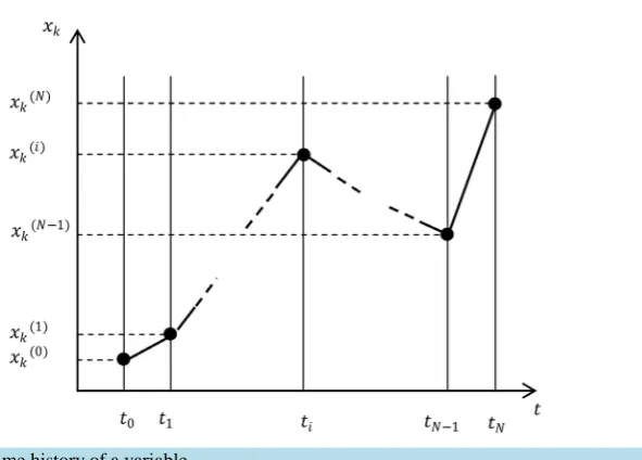
This idea can be extended to obtain an expected value of a m-dimensional functional that consists of m N× functions of time in the following way. First, independent variable t is divided by N, and x_k( )i values at time

i

[image:4.595.145.486.88.261.2]

Figure 1.Paths generated by a probability distribution.

Figure 2.Time history of a variable.

Note that the subscript k shows the k-th variable

(

1≤ ≤k m

)

. From Equation (4), the expected value

( )i k

x of x_k at t_i

(

0≤ ≤i N

)

is expressed as follows:

( ) ( ) ( )

_{( )}

( )

_{( )}

( )

_{( )}

( ) ( ) ( ) ( )

1 2

0 1

d d .

,

d

i i

k k

i i i i

m

N

x x P Dx t Dx t Dx t

Dx x x x

∞

−∞  

= _ ⋅ _

= ⋅

∫





(5)

The integral range is from −∞ to ∞ in Equation (5) according to the form of the path integral. The range in actual calculation is between the upper and lower limits of each variable. Also, Equation (5) is formulated to set the values according to the probability distribution for variable x_k( )i at time 0 and N. However, a variable may be fixed in some problems. The end points should be set in accordance with the boundary conditions.

Note that since Equation (5) shows the multiple integral, the Monte Carlo method can be applied to actual numerical calculations.

4. Calculation Algorithm for SPOT

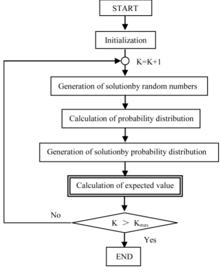
[image:4.595.186.482.284.496.2]

generated at a high frequency, and a solution with a poor performance index value is generated at a low fre-quency. Also, the algorithm is based on the Markov process so that future solutions will have no dependency on the former solutions. Lastly, expected values are calculated using all the solutions generated with a probability distribution to obtain an approximate solution.

The procedure of calculation is shown in Figure 3.

1) The values of all the variables are generated randomly to obtain initial solutions.

2) Time point t_i is chosen according to a random number, and function value x_i at t_i is randomly rewrit-ten to generate a different solution.

3) The performance index value of the newly generated solution is calculated.

4) The adoption or rejection of this solution is decided to generate solutions depending on the probability dis-tribution of Equation (3).

The procedure from Steps 2) to 4) is a pure explanation of the Metropolis method [7] to merely conduct the multiple integral. This method has an advantage of no necessity to obtain the normalization constant: A in Equation (3). A prime characteristic of this method is to calculate the expected values in Step 5).

5) The expected value is calculated.

6) If the final condition is met, the calculation ends. If not, it returns to the generation of solutions.

The final condition can be a certain range of variation of an expected value. However, in this paper, the final condition is the number of iterations, K_max. This is because the generation of solutions during the calculation is a Markov process, and therefore, the still more iterations of calculation can result in fine performance index values if the convergence of expected values is not enough.

[image:5.595.202.422.434.706.2]

Equation (3) for probability distribution in this paper is the same as that in SA. SA is a deterministic approach to search only optimal solution at h→0. On the other hand, h is finite and an optimal solution is obtained as an expected value (stochastic average value) in this paper. It means that the two approaches are based on funda-mentally different concepts. In the concrete, SA starts a search with an initial solution for candidate solutions according to the probability distribution. It adopts a solution of the best performance function value as an optim-al solution. On the other hand, our method determines an approximate solution to an optimoptim-al solution as an ex-pected value with all the solutions generated according to the probability distribution. In this method, there is no process of the so-called cooling schedule which is in SA.

5. Calculation Example

This section describes examples of numerical calculation with SPOT to demonstrate the validity. First, SPOT is applied to a problem where the minimum value of a multi-peaked function is obtained without staying at other minimal values and the minimum value is always only one with no dependency on the initial value. Next, we apply SPOT to a problem of obtaining the minimum value of a functional to show the validity in a physical op-timization problem. Lastly, we apply SPOT to an engineering optimal problem on the glide of a hang glider to show the high applicability of an approximate solution by SPOT.

We already applied SPOT to some engineering problems [8] [9].

5.1. Minimization Problem of Bivariate Function

First, we apply SPOT to a problem of obtaining the minimum value of a bivariate function expressed in Equa-tion (6). Here, performance funcEqua-tion I is the function value f x y

( )

, as follows:

(

,

)

{

cos 2π

(

)

cos 2.5π

(

)

2.1

}

{

2.1 cos 3π

(

)

cos 3.5π

(

)

}

, 0.0 3.0, 0.0 1.5

f x y = x + x − × − y − y ≤ ≤x ≤ ≤y (6)

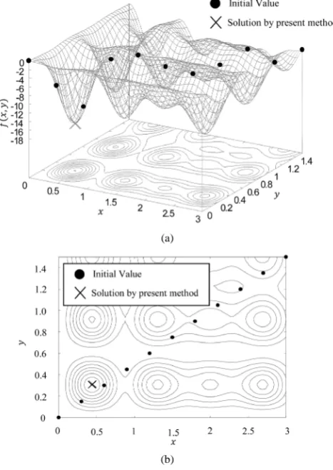
Figure 4(a) shows the solution space of Equation (6). The set of f x y

( )

, that minimizes this function is

(0.439, 0.306). This function has multiple minimal values and thus is a multi-peaked function. The contours are shown in the bottom plane, and Figure 4(b) shows the top view.

This example is a problem for obtaining the minimum value of a bivariate function. Therefore, the variables are not discretized, but the values of two variables are generated according to the probability distribution (3) de-fined by the performance values to obtain an expected value. The closed dots in Figure 4(a) show multiple ini-tial values chosen to check the dependency on the iniini-tial values. Also, the cross marks in Figure 4(b) show the minimum values obtained with this method.

(a)

[image:6.595.195.429.377.707.2]

(b)

If calculation starts with any initial value marked in the closed dot, the resultant values do not stay at any of the many minimal values in the solution space, but all the values concentrate near the minimum value. Since every solution generated in each calculation is obtained stochastically with this method, the calculation results are not influenced by the initial value in principle. However in reality, the number of calculations is finite. Therefore, the expected value as the minimum value may have a variation. The minimum values in Figure 4(b) have a little variation though it may be invisible. This variation is caused by the limited number of calculations.

Note that it took about 18 seconds to perform one million times of calculations on a 1.4 GHz Pentium 4 ma-chine.

5.2. Line of Swiftest Descent Problem

Next, we applied SPOT to a problem on brachistochrone as one of the classical optimization problems to obtain a function. This problem is demonstrated to obtain a mass point path that shows the brachistochrone between a fixed start point and an end point at different altitudes under the uniform gravitation field. Here, performance function I is time t until the mass point reaches the end point as expressed in the following equation:

(

)

2

0

1 d d

1

d 2

f

y x y

t y

g y

+

=

_∫

. (7)

The boundary conditions are as follows:

Initial condition: y

( )

0 =x

( )

0 =0, final condition:y t

( )

_f =1.0, x t

( )

_f =π 2.

In this problem, we discretized the vertical axis y at an even division, and generate the values of the hori-zontal axis x corresponding to y according to the probability distribution of Equation (3) defined by the performance index of Equation (7) to obtain an expected value.

Figure 5 shows the paths obtained with SPOT in the closed dots and the analytic solution in the solid line. It took about 438 seconds on a Pentium 4 machine to perform 20 million times of iterations.

SPOT is to obtain an approximate solution of an optimal solution. However, the approximate solutions agree well with the analytic solutions. Thus, this method can be applied to general optimization problems where per-formance functions are expressed in functional.

5.3. Optimal Glide Problem of Hang Glider

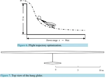
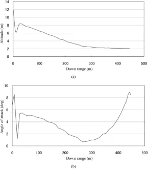
Lastly, we apply SPOT to a problem of a hang glider that starts the fall and glide at an altitude of 12 m toward the ground to obtain its flight operation (time history of angle of attack) for the maximum down range (as shown in Figure 6).

This problem was firstly solved by Suzuki et al. [10] and their results were used to check the validity of the results of SPOT.

[image:7.595.158.471.552.713.2]

This problem is based on the former problem of [10] and the specifications of the hang glider used here are based on those of the optimal glider obtained in [10]. The shape of the hang glider is shown in Figure 7.

[image:8.595.141.488.86.341.2]

Figure 6.Flight trajectory optimization.

Figure 7.Top view of the hang glider.

Note that the performance index is the reciprocal number of the flight distance to set this problem to a minim-al vminim-alue problem. Also, the maximum vminim-alue of the load factor is set to the restriction condition. If this condition exceeds the limitation during the flight, a penalty is added to the performance index value.

The equation of motion is as follows:

(

)

2

1

1 2 D sin

V= − m ρV S C∗ −g γ , (8)

(

1 2m

)

VS C1 L

(

g V

)

cos

γ_= ρ ∗₋ γ

, (9)

cos

x=V

γ

(10) sin

z=V γ (11)

The main conditions are shown as follows: Performance index:

max

1

i

f i f

n n

I x n x

>

= +

∑

(12)

Initial condition: z₀=12.0 m, V₀=5.0 m/s, γ = −₀ 3.5 deg. Final condition: z_f =2.0 m.

Restriction condition: n_max =3.0.

Specifications of hang glider: S₁=14.6 m2, A₁=36.0, b₁=22.9 m, λ =₁ 0.5, S₂=2.3 m2, A₂ =6.0,

2 0.5

λ = , m₀ =35.0 kg, m_p=60.0 kg.

The performance index value is the reciprocal number of the down range at the point where the hung glider reaches at an altitude of 2 m. First, the control variable, which is the angle of attack in this case, is discretized on the axis of time. Next, values of angle of attack at each time are specified with random numbers. The equations of motion are numerically calculated according to the time history of angle of attack to obtain the flight path. Then, the performance index value is determined as a reciprocal number of the down range. Therefore, the per-formance index values are obtained when the series of calculations ends with the final conditions being met.

Figure 8(a) and Figure 8(b) show the relation between the down range and the altitude, and that between the down range and the angle of attack, respectively.

(a)

[image:9.595.168.461.90.423.2]

(b)

Figure 8.(a) Altitude vs. down range; (b) Angle of attack vs. down range.

6. Discussion

We propose a new optimization method with a stochastic process called SPOT, and then demonstrate numerical calculations.

Generally, when proposing a new method, comparison of performance between the conventional method and a new method should be performed. However, since SPOT is the only method of obtaining the approximate value of the optimal solution, there is no sense in comparing them. Also fair comparison of computation time could not be performed.

As a result, SPOT has the following characteristics:

1) Advantages of Stochastic Process

SPOT results in an expected value from all the solutions generated by calculations. One of the advantages is to avoid influences from the initial value (a start point of the calculation) to the final expected value. The reason is that the generation of solutions during the calculation is a simple stochastic process, and the initial value is only the first-generated solution. As shown in Section 6.1, the calculation results all do not stay at local minimal values even though the calculation starts with any initial value, but the resultant values concentrate near the minimum value. Another advantage is to update an expected value from optimal solutions separately obtained under the same condition. This enables a parallel calculation and the recycling of the former calculation results. This characteristic is unique to SPOT and advantageous to other numerical calculation methods. For example, the calculation of a bivariate function, as shown in Section 6.1, gives the results starting with the multiple initial points as different minimum values. (The cross marks actually show almost the same point.) On the other hand, it is possible to obtain an expected value with all these expected values.

time can easily be estimated with the number of calculations. Therefore, it is easy to estimate the calculation cost.

2) Independency on Experience

Another characteristic is that SPOT has only fluctuation parameter, h, set by operators. There may be a case of extremely low convergence of a solution because of a large fluctuation during calculation with an conven-tional optimization method using an inclination of the solution curved surface if the features of the solution space are not well known. On the other hand, in principle, the scale of the fluctuation parameter in our method has almost no influence on the process of obtaining an expected value. Although variations of convergence times of calculations due to the scale of the parameter are observed in actual calculations with the limited number of calculations, any large influence on the obtained expected values has not been known. Therefore, this method can be applied to unknown problems, including the surroundings, on solution spaces.

Also, the smaller the fluctuation parameter during calculation, the shorter the calculation time is, though this characteristic is not mentioned in this paper.

3) Restriction Conditions

In the conventional calculation approaches that start with initial solutions to search better performance index values, it may be difficult to generate an initial solution itself and thus to start the numerical calculation if the solution space is narrowed with restriction conditions. However, since the generation of solutions during calcu-lation in our method is a stochastic process, it is possible to perform the calcucalcu-lation regardless of the presence of solutions.

Also, if there are restriction conditions on parameters, which are not the fluctuation parameter: h in (b) but are the load factor: n and the angle of attack: α etc. in Section 6.3 for example, it is necessary to keep pa-rameters within the restriction conditions with general methods. However, with our method, such a device is not necessary. Furthermore, the restriction conditions are rather advantageous to numerical calculations. For exam-ple, if there are restrictions on parameter values and the range is specified, solutions can be generated only with values within the restrictions in the process where the series of solutions are generated. This is largely advanta-geous to perform numerical calculations. The harder the restriction conditions are and the narrower the range of the resultant parameter values is, the more densely the solutions are generated within the restriction conditions and the more easily the calculations are.

Next, in case of restriction conditions on state variables, when a solution generated during calculation is trapped on the restriction, the solution may be abandoned. However, expected values may approach but do not reach the restriction surfaces using only parameter values within constraint ranges and abandoning solutions that break the restrictions. Parameters and solutions that break the restrictions can be applied to a calculation using a penalty method to approach the expected value toward the restriction surface more closely. However, if results with this method are used as initial solutions of deterministic approaches, there is no necessity to make a device.

4) Scope of SPOT

The characteristics of SPOT are to obtain expected values of solution spaces with multiple integral. Thus, there is no problem if the solution spaces have restrictions as mentioned above. However, SPOT is not appropri-ate to be used for problems that have no restriction on the infinite solution spaces. Also, if a problem has a large solution space and a sharp peak on the performance index value, this method can be applied in principle. How-ever, it may be difficult to obtain an approximate solution with high accuracy in the finite number of calculations. However, it is rare to have infinite range of a variable in an engineering problem, and the upper and lower limits can generally be set. Also, the fluctuation of a performance index value to that of a variable is expected to be smooth. Furthermore, the accuracy required for a variable is finite. Therefore, it is possible to obtain an ap-proximate value for practical use with the finite number of calculations.

7. Conclusions

We propose a new optimization method based on the path integral called SPOT, and thus perform a numerical calculation on an engineering optimization problem. As a result, we obtain an approximate value of an optimal solution with high accuracy. In addition, this stochastic method has advantages on numerical calculation to other methods.

References

[1] Kirkpatrick, S., Gelatt Jr., C.D. and Vecchi, M.P. (1983) Optimization by Simulated Annealing. Science, 220, 671-680. http://dx.doi.org/10.1126/science.220.4598.671

[2] Terasaki, M., Kondo, M., Yoshida, H., Yamaguchi, K. and Ishikawa, Y. (2004) Integrated Optimization of Airplane Design and Flight Trajectory by New Optimization Method Using a Stochastic Process. In: CONPUTATIONAL MECHANICS WCCM VI in Conjunction with APCOM’04, Tsinghua University Press & Springer-Verlag, Beijing, 328.

[3] Yoshida, H., Konno, T., Yamaguchi, K. and Ishikawa, Y. (2005) New Optimization Method Using Stochastic Process Based on Path Integral. Journal of the Japan Society for Computational Methods in Engineering, 5, 145-150. (in Japa-nese)

[4] Yoshida, H., Yamaguchi, K. and Ishikawa, Y. (2006) Application of a New Optimization Method for System Design. Joint 3rd International Conference on Soft Computing and Intelligent Systems (SCIS) and 7th International Symposium on Advanced Intelligent Systems (ISIS), Tokyo, 20-24 September 2006, 1542-1547.

[5] Yoshida, H., Yamaguchi, K. and Ishikawa, Y. (2007) Design Tool Using a New Optimization Method Based on a Sto-chastic Process. Transactions of the Japan Society for Aeronautical and Space Sciences, 49, 220-230.

http://dx.doi.org/10.2322/tjsass.49.220

[6] Feynman, R.P. and Hibbs, A.R. (1965) Quantum Mechanics and Path Integrals. McGraw-Hill, New York.

[7] Metropolis, N., Rosenbluth, A.W., Rosenbluth, M.N., Teller, A.H. and Teller, E. (1953) Equation of State Calculations by Fast Computing Machines. Journal of Chemical Physics, 21, 1087-1092. http://dx.doi.org/10.1063/1.1699114

[8] Nakane, M., Kobayashi, D., Yoshida, H. and Ishikawa, Y. (2009) Feasibility Study on Single Stage to Orbit Space Plane with RBCC Engine. 16th AIAA/DLR/DGLR International Space Planes and hypersonic Systems and Technolo-gies Conference, Bremen, AIAA 2009-7331. http://dx.doi.org/10.2514/6.2009-7331

[9] Ishimori, Y., Nakane, M., Ishikawa, Y., Yoshida, H. and Yamaguchi, K. (2011) Feasibility Study for Spaceplane’s Concepts in Ascent Phase Using the Optimization Method. Journal of the Japan Society for Aeronautical and Space Sciences, 59, 291-297. (in Japanese) http://dx.doi.org/10.2322/jjsass.59.291

Nomenclature

1

A = wing aspect ratio;

1

A∗= wing aspect ratio including the ground effect

{

33

(

z b₁

)

3 2+1

}

33

(

z b₁

)

3 2;

1

b = wing span;

L

C = lift coefficient;

0 D

C = parasite drag coefficient C_DW0+C_Df S_f S₁+C_DrW0S₂ S₁;

Df

C = fuselage drag coefficient;

0 DW

C = wing minimum drag coefficient;

0 DrW

C = horizontal stabilizer minimum drag coefficient;

D

C∗ = drag coefficient including the ground effect C_D0+C_Di∗ ;

L

C∗ = lift coefficient including the ground effect C A_{L 1}∗ A₁;

Di

C∗ = induced drag coefficient including the ground effect C_L∗2 πeA₁∗; e= Oswald’s airplane efficiency;

g= gravitational constant;

m= total mass m₀+m_p;

0

m = mass of the hung glider;

p

m = mass of the pilot;

i

n = load factor at i-th discrete time;

1

S = wing area;

2

S = horizontal stabilizer area;

f

S = fuselage representative area; t= time;

f

t = final time; V = speed;

x= position, down range;

f

x = down range at the end point; y= position;