http://dx.doi.org/10.4236/am.2015.62034
Availability Importance Measures for
Virtualized System with Live Migration
Junjun Zheng, Hiroyuki Okamura, Tadashi DohiDepartment of Information Engineering, Graduate School of Engineering, Hiroshima University, Higashi-Hiroshima, Japan
Email: [email protected], [email protected], [email protected]
Received 16 January 2015; accepted 6 February 2015; published 10 February 2015
Copyright © 2015 by authors and Scientific Research Publishing Inc.
This work is licensed under the Creative Commons Attribution International License (CC BY). http://creativecommons.org/licenses/by/4.0/
Abstract
This paper presents component importance analysis for virtualized system with live migration. The component importance analysis is significant to determine the system design of virtualized system from availability and cost points of view. This paper discusses the importance of compo-nents with respect to system availability. Specifically, we introduce two different component im-portance analyses for hybrid model (fault trees and continuous-time Markov chains) and conti-nuous-time Markov chains, and show the analysis for existing probabilistic models for virtualized system. In numerical examples, we illustrate the quantitative component importance analysis for virtualized system with live migration.
Keywords
Virtualized System, Live Migration, System Availability, Component Importance Analysis, Fault Tree, Continuous-Time Markov Chain
1. Introduction
they can be migrated to another physical server running the virtualization platform. In particular, if two physical servers have the same platform that can drive virtual machines, we exploit the live migration between them [2]. The live migration is a technique that allows a server administrator to move a running virtual machine of appli-cation between different physical machines without disconnecting the client or appliappli-cation. The live migration drastically improves the system availability by migrating a failed virtual machine on a platform to another plat-form.
Although the virtualization is a promising way for HA services, the design of system architecture is not so easy, compared to non-virtual system. For example, the system availability can easily be improved by increasing physical servers which run the virtualization platform. However, from the points of cost and energy consump-tion, it is not always the best design. That is, towards the best design of virtualized system, we should consider the method to evaluate the system performance beforehand.
On the performance index, Kundu et al. [3] presented statistical models using regression and artificial Neural networks. Also, Okamura et al. [4] proposed a queueing model to evaluate energy efficiency of virtualized sys-tem design. On the syssys-tem index for reliability and availability, Cully et al. [5] and Farr et al. [6] built and eva-luated their schemes to enhance the system availability in virtualized system design. Myint and Thein [7] also evaluated a system architecture combining virtualization and rejuvenation. Vishwanath and Nagappan [8] col-lected operation data of virtualized system and performed statistical analysis to reveal a causal relationship be-tween server failures and hardware repairs. Kim et al. [9] focused on failure modes of virtualized system and presented availability evaluation using fault trees and continuous-time Markov chains (CTMCs). Also Matos et al. [10] developed the CTMC model representing the dynamic behaviors of live migration in the virtualized system. Zheng et al. [11] considered the component importance analysis for non-virtualized and virtualized sys-tem based on the model by Kim et al. [9].
This paper is an extension work of [11]. In [11], we have developed a method to evaluate the importance (the effect of a component’s availability on the system availability) of components for hybrid models. The hybrid model consists of fault trees (FTs) and CTMCs. The FTs are top level descriptions for the system failure and represent causal relationship between component failures and system failures. The disadvantage of FT is not to describe the dynamic behaviors. To address this problem, dynamic FT is also proposed in [12]. On the other hand, CTMC can well describe the dynamic behaviors of system. In the hybrid model, CTMCs are used for de-fining the behavior of components. The advantage of hybrid model is to obtain the structure function of system failure with respect to component failures from FT and to be able to define the dynamic behaviors of compo-nents. Based on this feature, we have proposed the component importance analysis for hybrid model in [11]. However, the hybrid model had a limitation for the model expression. For example, when two or more compo-nents have interactions between them, the structure function cannot always be explicitly expressed. In such cases, we cannot use the hybrid model. Instead of using the hybrid model, we should use a CTMC describing whole the system behavior. In the component analysis of virtualized system, the behavior of live migration is this case. In fact, Matos et al. [10] presented only a CTMC for the live migration. Since the structure function cannot be obtained from the CTMC, we cannot also apply the component importance analysis by [11] to the live migration model. In this paper, we introduce the state-of-art component importance analysis [13] and apply it to the CTMC-based live migration model to reveal the component importance in the context of live migration.
The rest of this paper is organized as follows. Section 2 presents the hybrid model for virtualized system de-sign in [11], and introduces the component importance analysis for the hybrid model from the availability point of view. In Section 3, we explain the CTMC model for live migration presented in [10], and show the compo-nent importance analysis by using only CTMCs. In Section 4, we illustrate the compocompo-nent importance analysis of hybrid model and live migration model for virtualized system. Section 5 concludes this paper with some re-marks.
2. Availability Importance Analysis for Hybrid Model
2.1. Fault Trees
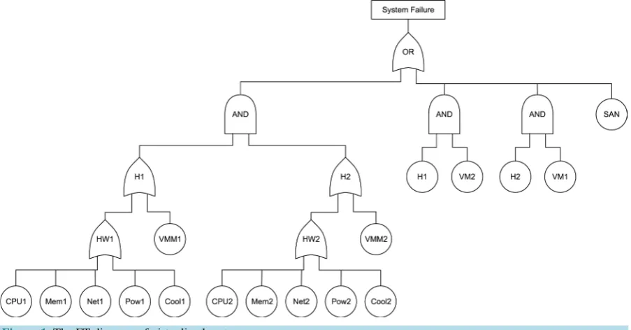
cooling subsystem (Cool) but also a software component; virtual machine manager (VMM).
Figure 1illustrates the fault tree (FT) for virtualized system when there are two physical hosts. In the system design, each host provides a specific service, and is supposed to install the same VMM where the virtual ma-chines (VMs) run and provide the services. One of the important features provided by the VMM is the live mi-gration [2]. The live migration is a technique that can enhance the system availability by migrating the VMs when system failure occurs. More precisely, when a physical host is stopped, all the VMs running on the host can migrate to another physical host without the down time. In fact, most of the VMM products such as Xen, VMware and Hyper-V provide the live migration. However, in order to use the live migration, the two hosts are required to share a common storage area network (SAN) which is a service to provide hard disk drives through a high-speed network using Fiber Channel or iSCSI technologies. In Figure 1, the top event means the system failure and the leaf nodes correspond to the events that respective components are failed. The nodes, H1 (H2) and HW1 (HW2) represent the events that the host 1 (host 2) is failed and the hardware failure occurs in the host 1 (host 2), respectively. The failure of the system is given by an AND gate because of the live migration. In ad-dition, the VM failure (VM1 or VM2) is connected to the failure of another host (H2 or H1) with an AND gate. This is because even if the VM is failed on one VMM, it can be migrated to another VMM. On the other hand, the failure of SAN causes the system failure directly, and therefore the top event is given by an OR gate con-nected to these events.
2.2. Continuous-Time Markov Chain (CTMC) Models
In [9], Kim et al. defined the continuous-time Markov chain (CTMC) models to represent behavior of hardware and software components. This section briefly introduces the CTMC models presented in [9].
In the availability modeling, the state of system can be classified into two sets: , the set of up (operational) states in which the system is available; and , the set of down (or failure ) states in which the system is un-available.Figure 2 shows the 3-state CTMC availability models of CPU and Mem components proposed in [9]. In the figure, the states UP, DN and RP mean that the component is available, the component is failed, and the component is under repair, respectively. Hence the states DN and RP are classified into set in the availabil-ity model. Moreover, λ and µ denote failure and repair rates of the component. For example, if the host equips 2-way CPUs, the failure rate is given by λ=2λCPU by using the failure rate of a single CPU because
both processors are needed for the operation. Also, the transition from DN to RP corresponds to the event that a repair person is summoned and its mean time is given by 1α using the rate of summoning inherent in the component.
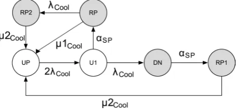
As seen inFigure 3, Kim et al.[9] applied the 5-state availability model to describe the dynamic behaviors of components Pow and Net which are described as 2-unit redundant (parallel) subsystems. In the figure, white and gray nodes represent up and down states respectively. The main difference from the 3-state availability model is to add the state U1 representing that only one unit is failed, since the component failure is caused when both of two units are failed. Moreover, the model adds a repair state RP2 where two units are failed. For the components, Cool and SAN, the CTMC models are extended from the 5-state availability model. Concretely, in the CTMC for Cool as shown inFigure 4, they added a transition from RP to RP2, namely, the Cool availability model al-lows the event occurrence that one unit fails while another unit is under repair. In the CTMC for SAN as shown inFigure 5, a state CP is put to the transition between the states UP and RP, which means the mirrored data is copied from a working disk unit to the repaired disk unit under RAID1 design. The transition rate from CP to UP is given by χSAN. Additionally, since the working disk unit may fail in the CP state, they added a transition
from CP to RP2 with the failure rate of a disk unit λSAN.
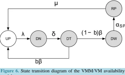
The CTMC model for VMM is given byFigure 6. As seen in this figure, since the software failure cannot be detected immediately, the state DT is added, which means the failure is detected. In [9], after the failure detec-tion, the system takes an action to reboot VMM with mean time 1 β. It is empirically known that most of tran-sient failures in software can be recovered by the system reboot [14]. In this CTMC model, the reboot will be unsuccessful with probability
(
1−b)
. Hence the state DW indicates that the failure is not recovered by a failed system reboot, and a repair person is summoned.In [9], based on the CTMC model inFigure 6, they built the CTMC model for VM which takes account of the dynamic behaviors of the live migration. Thus the CTMC model for VM was quite complicated so that the
[image:4.595.140.486.337.404.2][image:4.595.218.413.433.543.2]
Figure 2. State transition diagram of the CPU and memory availability models.
Figure 3.State transition diagram of the power (or network card) availability model.
[image:4.595.194.435.582.693.2]Figure 5. State transition diagram of the SAN availability model.
Figure 6. State transition diagram of the VMM/VM availability model.
system failure in the virtualized system cannot be represented by the FT. Since this paper describes the correla-tion between the failures of VM and host by the AND gate in the FT representacorrela-tion, the CTMC model simply becomes the same model as VMM, i.e., the model ofFigure 6 can also represent the availability for VM.
Based on these CTMC models, the steady-state availability for component x can be calculated as follows.
[
)
the cumulative available time during 0, lim
x k
t
k
t A
t π
→∞ ∈
= =
∑
(1)
where πk is the steady-state probability of state k in the availability model and is the set of up states. The steady-state probability πk is computed by numerical methods given in [15].
2.3. Importance Measures
Let Ai be the steady-state availability of component i. Then we have the following steady-state availability for a host in the virtualized system according to the FT analysis:
VMM HW
,
H i
i
A A A
∈
=
∏
(2)where HW is the set of
{
CPU, Mem, Net, Pow, Cool}
. Then the system availability can be obtained(
)
(
H1 H2 H1 VM2 H2 VM1 H1 H2 VM2 VM1)
(
SAN)
1 1 ,
S
A = − A A +A A +A A −A A A +A −A (3)
where Ai= −1 Ai. The above equation is often called the structure function which represents the effect of com-ponent availability on the system availability.
[image:5.595.193.433.240.384.2], ,
1 1
, ,
S S
i i
S i S i
A A
I I
A A
λ λ µ µ
∂ ∂
= =
∂ ∂ (4)
where λi and µi are the failure and repair rates of component i, i.e., the transition rates from up to down and from down to up in the 2-state availability model, respectively. These measures come from the idea behind the Birnbaum measure [17].
In this paper, since we do not treat the 2-state availability model to represent the component availability, the importance measures proposed in [16] cannot directly be applied to evaluating the virtualized system. This paper proposes a preprocessing based on the aggregation of CTMC-based availability model [18] before applying the availability importance measures.
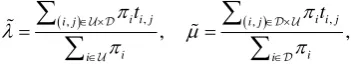
The aggregation is a technique to transform CTMC-based availability models into a equivalent 2-state, 2-transition availability model which has the same availability as the original model. As mentioned before, the states of CTMC-based availability models can be classified into (up states) and (down states) sets. The aggregation technique converts the and sets to the up and down states of the equivalent 2-state, 2-transition availability model. The essential problem of the aggregation is to find the transition rates; failure and repair rates that ensure the steady-state probability of the up (down) set in the original model equals that of the up (down) state in the equivalent 2-state, 2-transition model. From the argument of CTMC, such failure and repair rates can be computed as follows.
( ), , ( ), ,
, ,
i i j i i j
i j i j
i i i i t t π π λ µ π π ∈ × ∈ × ∈ ∈ =
∑
=∑
∑
∑
(5)where the set × indicates the transitions from up to down state in the original model. Also, ti j, denotes
the transition rate from state i to state j in the original model. For simplification, ti j, =0 if there is no transition
from state i to state j. The calculated failure and repair rates λ and µ in the equivalent 2-state, 2-transition availability model are called the equivalent failure and repair rates [18]. In this paper, we call the equivalent failure and repair rates as the effective failure and repair rates.
By applying the aggregation to the component availability models as preprocessing, the availability impor-tance measures of the component i can be rewritten by
, , 1 1 , , S S i i
S i S i
A A
I I
A µ A
λ λ µ
∂ ∂
= =
∂ ∂
(6)
where λi and µi are the effective failure and repair rates of component i.
3. Component Importance for Live Migration
In the previous section, we have introduced the component importance for the structure function given by the FT model. The model considered the live migration as a static structure. However, since the live migration is essen-tially described by a dynamic behavior, the previous method cannot analyze how effect of components on the dynamic behaviors of live migration. Thus in this section, we consider the component importance on live migra-tion from the viewpoint of dynamic behaviors, that is, we apply the component importance analysis for a CTMC representing the dynamic behaviors of live migration presented in [10].
3.1. Model Description
Matos et al. [10] presented the CTMC for live migration in the virtualized system. This availability model does not consider the detailed behavior of hardware components (e.g., CPU, Mem, Pow) and the VMM, but only the components of VMs (VM1 and VM2), hosts (H1 and H2) and applications (App1 and App2).
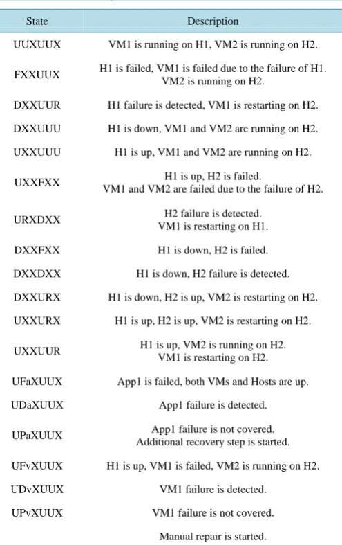
[image:6.595.219.395.308.341.2]Table 1. The states of system.
State Description
UUXUUX VM1 is running on H1, VM2 is running on H2.
FXXUUX H1 is failed, VM1 is failed due to the failure of H1.
VM2 is running on H2.
DXXUUR H1 failure is detected, VM1 is restarting on H2.
DXXUUU H1 is down, VM1 and VM2 are running on H2.
UXXUUU H1 is up, VM1 and VM2 are running on H2.
UXXFXX H1 is up, H2 is failed.
VM1 and VM2 are failed due to the failure of H2.
URXDXX H2 failure is detected.
VM1 is restarting on H1.
DXXFXX H1 is down, H2 is failed.
DXXDXX H1 is down, H2 failure is detected.
DXXURX H1 is down, H2 is up, VM2 is restarting on H2.
UXXURX H1 is up, H2 is up, VM2 is restarting on H2.
UXXUUR H1 is up, VM2 is running on H2.
VM1 is restarting on H2.
UFaXUUX App1 is failed, both VMs and Hosts are up.
UDaXUUX App1 failure is detected.
UPaXUUX App1 failure is not covered.
Additional recovery step is started.
UFvXUUX H1 is up, VM1 is failed, VM2 is running on H2.
UDvXUUX VM1 failure is detected.
UPvXUUX VM1 failure is not covered.
Manual repair is started.
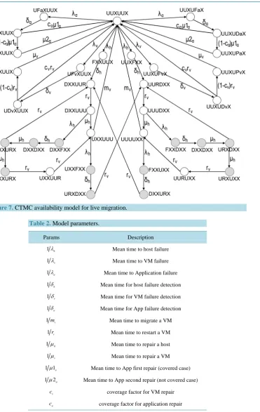
state of system is represented by “Da”. If App1 requires an additional repair in the case where the application restart cannot solve the problem, the character is given by “Pa”. Also, when VM1 and App1 are restarting, the state is given by “R”. If VM1 and App1 are not running on the H1, then the character is “X”. The third character represents whether or not VM2 and App2 are running on H1. If VM2 and App2 run on H1, the character is giv-en by “U”. If they are restarting on H1, the character is “R”. Otherwise, if they are not running on H1, the cha-racter is “X”. The fourth through sixth chacha-racters represent the state of H2 in the same manner as the first through third characters.Figure 7 shows the state transition diagram for live migration in the virtualized system which is described by the CTMC model in [10]. Also,Table 2 presents the parameters of the CTMC model. For example, 1λh is MTTF (mean time to failure) of host H1 and H2, and then λh is a failure rate which is a transition rate in the CTMC.
3.2. Importance Analysis
Dissimilar to the case of FT model, we do not know the structure function in the CTMC. We consider the com-ponent importance analysis by only using the parameter sensitivity analysis.
Let Q be the infinitesimal generator of CTMC described inFigure 7. Then the steady-state probability vector
πs is given by the linear equations;
, 1,
s = s =
Figure 7. CTMC availability model for live migration.
Table 2. Model parameters.
Params Description
1λh Mean time to host failure
1λv Mean time to VM failure
1λa Mean time to Application failure
1δh Mean time for host failure detection
1δv Mean time for VM failure detection
1δa Mean time for App failure detection
1mv Mean time to migrate a VM
1rv Mean time to restart a VM
1µh Mean time to repair a host
1µv Mean time to repair a VM
1µ1a Mean time to App first repair (covered case)
1µ2a Mean time to App second repair (not covered case)
v
c coverage factor for VM repair
a
c coverage factor for application repair
[image:8.595.126.519.80.370.2]• ξsys: a 0 - 1 vector whose elements are 1 in the state where the system is up.
Then the component availability is given by a inner product of πs and ξ⋅; for example, the component availa-bility of H1 becomes
1 1. h s h
A =π ξ (8) On the other hand, the system availability can be obtained by
. S s sys
A =π ξ (9)
Similar to the case of FT model, we define the importance measures of component i as follows.
, , 1 1 , , S S i i
S i S i
A A
I I
A µ A
λ λ µ
∂ ∂
= =
∂ ∂
(10)
where λi and µi are the effective failure and repair rates of component i. They can be computed by the ag-gregation technique introduced in Section 2.3. Also, we have
(
)
, 2
1 1 1
.
S S i S i
i
S i S i i S i i i
A A A A
I
A A A A A
λ
µ
λ λ λ µ
∂ ∂ ∂ ∂
= = =
∂ ∂
∂ ∂ +
(11)
Similarly, the importance measure with respect to repair rate is given by
(
)
, 2 1 . S i i S i i i A I A A µ λ λ µ ∂ = ∂ + (12)
Thus the problem is to estimate the sensitivity ∂AS ∂Ai without the structure function.
To estimate the sensitivities for all the component availabilities, we consider the sensitivities of system and component availabilities with respect to model parameters. Suppose that θ1,,θm are model parameters of the underlying CTMC. Here we define a matrix J and a column vector z whose elements are the sensitivities for all the component availabilities and the system availability with respect to the model parameters, i.e.,
1 2
1 1 1 1
1 2
2 2 2 2
1 2
, ,
n S
n S
n S
m m m m
A A A A A A A A A A A A
θ θ θ θ
θ θ θ θ
θ θ θ θ
∂ ∂ ∂ ∂ ∂ ∂ ∂ ∂ ∂ ∂ ∂ ∂ ∂ ∂ ∂ ∂ = = ∂ ∂ ∂ ∂ ∂ ∂ ∂ ∂ J z (13)
where A1,,An represent component availabilities for all the components. These sensitivities can be obtained by solving the following linear equations:
( )
j s,( )
j s ,( )
j 0.j j
θ θ θ
θ θ
∂ ∂
= = − =
∂ ∂
s π s Q π Q s 1 (14)
By using the vector s
( )
θj , the sensitivities are given by( )
,( )
.i S
j i j sys
j j
A θ A θ
θ θ
∂ = ∂ =
∂ s ξ ∂ s ξ (15)
According to [19], the estimates of ∂AS ∂Ai can be obtained by
( )
T 1 T T 1 2 = ,S S S
n
A A A
A A A
−
∂ ∂ ∂
∂ ∂ ∂
J J J z (16)
4. Numerical Illustration
4.1. Hybrid Model
In this section, we illustrate the quantitative component importance analysis of hybrid model for virtualized sys-tem.Table 3 presents the parameters of the CTMC models for all components. For example, 1λCPU is mean
time for CPU failure, and 1µMem is mean time to repair one memory (i.e., MTTR of one memory). Also we
give other model parameters inTable 4.
Using the aggregation technique, we first transform the availability models for all components into the equiv-alent 2-state, 2-transition models, then compute the effective failure and repair rates for components based on the model parameters. We also compute the component availabilities, and these results are shown inTable 5. From this table, we can see the availabilities of hardware units are relatively high by the comparison to the availabilities of software components, especially for SAN, the availability is quite high.
We then compute the system availabilities based on the structure functions and the component availabilities. The availabilities of a hardware unit and a host, and the system availability are presented inTable 6. From this table, the sufficiently high availability of the virtualized system implies that the live migration is considerably effective to enhance the system availability.
[image:10.595.187.439.357.719.2]Next we derive the importance measures of components in the virtualized system by using Equation (6), and the effective failure and repair rates shown inTable 5. The importance measures of components in terms of the system availability are shown inTable 7. Note that this table presents the importance measures of components only in a host, because the components of the host 1 and 2 are assumed to be the same in the system design, and the importance measures of same components in the host 1 and 2 are identical.
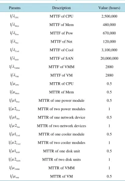
Table 3. MTTF/MTTR of components.
Params Description Value (hours)
CPU
1λ MTTF of CPU 2,500,000
Mem
1λ MTTF of Mem 480,000
Pow
1λ MTTF of Pow 670,000
Net
1λ MTTF of Net 120,000
Cool
1λ MTTF of Cool 3,100,000
SAN
1λ MTTF of SAN 20,000,000
VMM
1λ MTTF of VMM 2880
VM
1λ MTTF of VM 2880
CPU
1µ MTTR of CPU 0.5
Mem
1µ MTTR of Mem 0.5
Pow
1µ1 MTTR of one power module 0.5
Pow
1µ2 MTTR of two power modules 1
Net
1µ1 MTTR of one network device 0.5
Net
1µ2 MTTR of two network devices 1
Cool
1µ1 MTTR of one cooler module 0.5
Cool
1µ2 MTTR of two cooler modules 1
SAN
1µ1 MTTR of one disk unit 0.5
SAN
1µ2 MTTR of two disk units 1
VMM
1µ MTTR of VMM 1
VM
Table 4. Other model parameters.
Params Description Value
SP
1α Mean time to repair person summoned 30 minutes
SAN
1χ Mean time to copy data 20 minutes
VMM
1δ Mean time for VMM failure detection 30 seconds
VM
1δ Mean time for VM failure detection 30 seconds
VMM
1β Mean time to reboot VMM 10 minutes
VM
1β Mean time to reboot VM 5 minutes
VMM
b Coverage factor for VMM reboot 0.9
VM
[image:11.595.186.442.292.446.2]b Coverage factor for VM reboot 0.95
Table 5. Effective failure and repair rates and component availabili-ties.
Component λi µi Ai
CPU 8.0000000e−7 1.0000000 0.99999920
Mem 8.3333333e−6 1.0000000 0.99999167
Net 1.6666528e−5 1.9999833 0.99999167
Pow 2.9850702e−6 1.9999970 0.99999851
Cool 6.4516108e−7 1.9999990 0.99999968
VMM 3.4722222e−4 3.0769231 0.99988717
VM 3.4722222e−4 7.0588235 0.99995081
SAN 9.9999992e−8 1.9999999 0.99999995
Table 6. Availabilities of hardware units, host and system.
System Availability
HW1 and HW2 0.99998072
H1 and H2 0.99986789
System availability 0.99999992
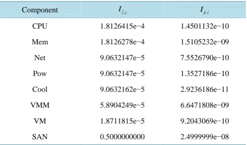
Table 7. Component importance measures in the virtualized system.
Component Iλ,i Iµ,i
CPU 1.8126415e−4 1.4501132e−10
Mem 1.8126278e−4 1.5105232e−09
Net 9.0632147e−5 7.5526790e−10
Pow 9.0632147e−5 1.3527186e−10
Cool 9.0632162e−5 2.9236186e−11
VMM 5.8904249e−5 6.6471808e−09
VM 1.8711815e−5 9.2043069e−10
[image:11.595.187.441.473.543.2] [image:11.595.187.442.571.720.2]Table 7shows that the importance measure with respect to failure rate is higher than that with respect to re-pair rate for any component. The importance measure regarding failure rate, Iλ,i, indicates the relative im-provement in system availability resulting from a decrease to the component failure rate. Similarly, the impor-tance measure regarding repair rate, Iµ,i, indicates the relative improvement in system availability resulting from an increase to the component repair rate. Thus, to improve the system availability, the more efficient way is to decrease the failure rates of components. Also, as seen in this table, it is easy to find that the importance measures of SAN are much higher than those of the other components, especially the importance measure with respect to failure rate, Iλ,SAN. The highest importance of SAN indicates that the improvement of failure rate of SAN is the most efficient way to improve the system availability. In other words, SAN is a bottleneck of availa-bility, though its availability seems to be high. Besides, fromTable 5, we find the repair rates of CPU and Mem are not so high. This implies that the failures of CPU and Mem cause long down time. Hence their importance measures with respect to failure rate are relatively higher than the others except SAN. Moreover, we find that the importance measures of VM and VMM are not high in Table 7. This is caused by the fact that VM and VMM can be migrated when a failure of a host occurs. Therefore, VM and VMM are not critical components, compared to SAN.
4.2. Dynamic Model for Live Migration
This section illustrates the quantitative component importance analysis of the CTMC for live migration in the virtualized system. Based on these parameters shown in Table 8, we first compute the availabilities for all components and system which are shown inTable 9. From this table, we find that the availability of VM is the highest among those of the other components because of the live migration.
Next we compute the effective failure and repair rates for all components based on the aggregation of CTMC model, and the results are shown inTable 10. From this table, it is found that the repair rate of VM are much higher than that inTable 5. As mentioned before, the FT model considered the live migration as a static struc-ture which cannot represent the dynamic behaviors of system. However, since the live migration is essentially described by a dynamic behavior, the dynamic behaviors have been taken into account in the CTMC model for live migration. The higher repair rate of VM confirms the effectiveness of live migration in the virtualized system.
Table 11presents the importance measures for components in the virtualized system. As observed inTable 10
Table 8. Model parameters.
Params Description Value
1λh Mean time for host failure 2654 hr
1λv Mean time for VM failure 2893 hr
1λa Mean time to Application failure 175 hr
1δh Mean time for host failure detection 30 sec
1δv Mean time for VM failure detection 30 sec
1δa Mean time for App failure detection 30 sec
1mv Mean time to migrate a VM 330 sec
1rv Mean time to restart a VM 50 sec
1µh Mean time to repair a host 100 min
1µv Mean time to repair a VM 30 min
1µ1a
Mean time to App first repair
(covered case) 1 min
1µ2a
Mean time to App second repair
(not covered case) 20 min
v
c Coverage factor for VM repair 0.95
a
Table 9. Availabilities of host, VM, application components and system.
System Availability
H1 and H2 0.9993644
VM1 and VM2 0.9999746
App1 and App2 0.9994520
System availability 0.9999992
Table 10.Effective failure and repair rates.
Component λi µi
H1 and H2 3.763673e−4 0.5917368
VM1 and VM2 7.212219e−4 28.351750
[image:13.595.184.443.104.399.2]App1 and App2 6.425198e−3 11.718790
Table 11. Component importance measures in the dynamic model for live migration.
Component Iλ,i Iµ,i
H1 and H2 2.118715e−03 1.347584e−06
VM1 and VM2 1.675414e−12 4.261977e−17
App1 and App2 9.438502e−13 5.174957e−16
andTable 11, we find that, although the failure rate of VM is higher than that of host, the importance measures of VM are much lower than those of host. This is because the repair rate of VM is very high. Also, comparing
[image:13.595.188.441.330.400.2]Table 9withTable 10, we can see that the availability of host is the lowest among those of others, because the repair rate of host is also the lowest. This indicates that, the component host is important, and any change in its associated parameters will have a large effect on the system availability. And this conclusion also can be con-firmed fromTable 11.
Table 11shows that the importance measures of host is the most highest. Moreover, by comparing between the importance measure with respect to failure and repair rates for each component, it is found that the impor-tance measure with respect to failure rate is higher than that with respect to repair rate. Therefore, it indicates that the improvement of failure rate of host is more efficient to enhance the system availability.
5. Conclusions
of reliability.
References
[1] Furht, B. and Escalante, A. (2010) Cloud Computing Fundamentals. In Handbook of Cloud Computing, Springer, 3-19.
http://dx.doi.org/10.1007/978-1-4419-6524-0_1
[2] Clark, C., Fraser, K., Hand, S., Hansen, J.G., Jul, E., Limpach, C., Pratt, I. and Warfield, A. (2005) Live Migration of Virtual Machines. In: Proceedings of the 2nd Conference on Symposium on Networked Systems Design & Implementa-tion—Volume 2, USENIX Association, Berkeley, 273-286.
[3] Kundu, S., Rangaswami, R., Dutta, K. and Zhao, M. (2010) Application Performance Modeling in a Virtualized Envi-ronment. Proceedings of the 16th IEEE International Symposium on High-Performance Computer Architecture, Ban-galore, 9-14 January 2010, 1-10.
[4] Okamura, H., Shigeoka, K., Yamasaki, K., Dohi, T. and Kihara, H. (2012) Performance Evaluation of Cloud Compu-ting in PaaS Environments. Supplemental Proceedings of 42nd Annual IEEE/IFIP International Conference on De-pendable Systems and Networks (DSN2012), 36, 122-127.
[5] Cully, B., Lefebvre, G., Meyer, D., Feeley, M., Hutchinson, N. and Warfield, A. (2008) Remus: High Availability via Asynchronous Virtual Machine Replication. Proceedings of the 5th USENIX Symposium on Networked Systems Design and Implementation, USENIX Association, Berkeley, 161-174.
[6] Farr, E., Harper, R., Spainhower, L. and Xenidis, J. (2008) A Case for High Availability in a Virtualized Environment (HAVEN). Proceedings of the 2008 Third International Conference on Availability, Reliability and Security (ARES'08), Barcelona, 4-7 March 2008, 675-682.
[7] Hla Myint, M.T. and Thein, T. (2010) Availability Improvement in Virtualized Multiple Servers with Software Reju-venation and Virtualization. Proceedings of 4th International Conference on Secure Software Integration and Reliabil-ity Improvement, Singapore, 9-11 June 2010, 156-162.
[8] Vishwanath, K.V. and Nagappan, N. (2010) Characterizing Cloud Computing Hardware Reliability. Proceedings of the first ACM Symposium on Cloud Computing (SoCC'10), Indianapolis, 10-11 June 2010, 193-204.
[9] Kim, D.S., Machida, F. and Trivedi, K.S. (2009) Availability Modeling and Analysis of a Virtualized System. Pro-ceedings of the 15th IEEE Pacific Rim International Symposium on Dependable Computing (PRDC-2009), Shanghai, 16-18 November 2009, 365-371.
[10] Matos, R.D.S., Maciel, P.R.M., Machida, F., Kim, D.S. and Trivedi, K.S. (2012) Sensitivity Analysis of Server Virtua-lized System Availability. IEEE Transactions on Reliability, 61, 994-1006.
[11] Zheng, J., Okamura, H. and Dohi, T. (2012) Component Importance Analysis of Virtualized System. Proceedings of the 9th IEEE International Conference on Autonomic & Trusted Computing (ATC2012), Fukuoka, 4-7 September 2012, 462-469.
[12] Cepin, M. and Mavko, B. (2002) A Dynamic Fault Tree. Reliability Engineering & System Safety, 75, 83-91.
http://dx.doi.org/10.1016/S0951-8320(01)00121-1
[13] Okamura, H., Zheng, J. and Dohi, T. (2015) Sensitivity Estimation for Markov Reward Models and Its Application to Component Importance Analysis. (In Submission)
[14] Castelli, V., Harper, R.E., Heidelberger, P., Hunter, S.W., Trivedi, K.S., Vaidyanathan, K. and Zeggert, W.P. (2001) Proactive Management of Software Aging. IBM Journal of Research and Development, 45, 311-332.
http://dx.doi.org/10.1147/rd.452.0311
[15] Trivedi, K.S. (2001) Probability and Statistics with Reliability, Queueing, and Computer Sciences Applications. 2nd Edition, John Wiley & Sons, New York.
[16] Cassady, C.R., Pohl, E.A. and Jin, S. (2004) Managing Availability Improvement Efforts with Importance Measures and Optimization. IMA Journal of Management Mathematics, 15, 161-174. http://dx.doi.org/10.1093/imaman/15.2.161
[17] Birnbaum, Z.W. (1969) On the Importance of Different Components in a Multicomponent System. In: Krishnaiah, P.R., Ed., Multivariate Analysis—II, Academic Press, New York, 581-592.
[18] Lanus, M., Yin, L. and Trivedi, K.S. (2003) Hierarchical Composition and Aggregation of State-Based Availability and Performability Models. IEEE Transactions on Reliability, 52, 44-52.http://dx.doi.org/10.1109/TR.2002.805781