Estimating SPT N value based on soil resistivity using hybrid ANN PSO algorithm

PAPER • OPEN ACCESS

Estimating SPT-N Value Based on Soil Resistivity

using Hybrid ANN-PSO Algorithm

To cite this article: Mohd Nur Asmawisham Alel et al 2018 J. Phys.: Conf. Ser. 995 012035

View the article online for updates and enhancements.

Related content

Comments and replies Ümit Gülerce

-Convertion Shear Wave Velocity to Standard Penetration Resistance A Madun, S A A Tajuddin, M E Abdullah et al.

-Statistical correlations of shear wave velocity and penetration resistance for soils

-Estimating SPT-N Value Based on Soil Resistivity using

Hybrid ANN-PSO Algorithm

Mohd Nur Asmawisham Alel1*, Mark Ruben Anak Upom1, Rini Asnida Abdullah1 and Mohd Hazreek Zainal Abidin2

1

Department of Geotechnics and Transportation, Faculty of Civil Engineering, Universiti Teknologi Malaysia, 81310 Johor Bahru, Johor, MALAYSIA

2

Faculty of Civil and Environmental Engineering, Universiti Tun Hussein Onn Malaysia, 86400 Batu Pahat Johor, MALAYSIA

E-mail: [email protected]

Abstract. Standard Penetration Resistance (N value) is used in many empirical geotechnical engineering formulas. Meanwhile, soil resistivity is a measure of soil's resistance to electrical flow. For a particular site, usually, only a limited N value data are available. In contrast, resistivity data can be obtained extensively. Moreover, previous studies showed evidence of a correlation between N value and resistivity value. Yet, no existing method is able to interpret resistivity data for estimation of N value. Thus, the aim is to develop a method for estimating N-value using resistivity data. This study proposes a hybrid Artificial Neural Network-Particle Swarm Optimization (ANN-PSO) method to estimate N value using resistivity data. Five different ANN-PSO models based on five boreholes were developed and analyzed. The performance metrics used were the coefficient of determination, R2 _{and mean absolute error,}

MAE. Analysis of result found that this method can estimate N value (R2

best=0.85 and

MAEbest=0.54) given that the constraint, Δ𝑙̅ref, is satisfied. The results suggest that ANN-PSO

method can be used to estimate N value with good accuracy.

1. Introduction

Standard penetration resistance test (SPT) has long been an industry standard for site investigation in the geotechnical field. The purpose of conducting SPT is to obtain the standard penetration resistance, commonly called the N value, which is the recorded blow count needed to advance through a 150 mm interval of soil. The N value provides engineers with a rough measure of the density of the soil and is used in many empirical geotechnical engineering formulas. However, a lot of construction project has started employing geophysical investigation as part of their site investigation process. Geophysical investigation such as electrical resistivity survey has a few advantages over more traditional site investigation methods like SPT such as non-destructive mapping technique, the ability to perform temporal monitoring of a particular site, various scales application, acquirement of detailed measurement over a large area with low cost and large sensitivity of the measurement [1].

1.1. Problem statement

covering a much larger volume although in the expense of accuracy. Previous studies showed evidence of a correlation between SPT-N and soil resistivity [2]. Sites possessing existing resistivity data usually have limited borehole data but an excess of resistivity data. Yet, no existing method is able to interpret resistivity data for estimation of N value.

1.2. Objectives

The objectives of this study are:

i) To determine potential application of ANN and PSO in the context of civil engineering. ii) To develop a computer program that can be used to solve an engineering problem using

ANN-PSO method.

iii) To facilitate estimation of N value using soil resistivity with measurable accuracy

1.3. Site layout

[image:3.595.99.321.351.526.2]

The data used in this research were obtained from a 2D resistivity survey conducted in Ulu Tiram, Johor. The borehole data used was down to the depth of 7.5 m. In addition, the site was composed of soil ranging from sand, silt, gravel and clay. Figure 1 shows the site layout while Table 1 shows the relative distance, l (m) and relative angle, Ɵ between the boreholes.

Figure 1. Site layout (aerial view) of borehole location together with geographic coordinate.

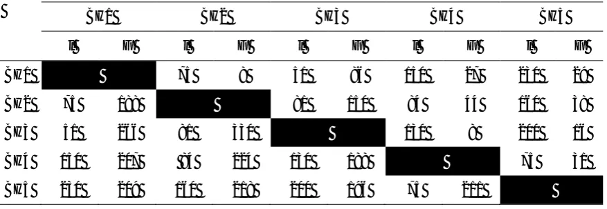
Table 1. Relative distance, l (m) and relative angle, Ɵ (ᵒ) between boreholes.

BH1 BH2 BH3 BH4 BH5

l Ɵ l Ɵ l Ɵ l Ɵ l Ɵ

BH1 75 8 51 86 150 27 230 29

BH2 75 188 81 150 84 44 160 38

BH3 51 266 81 330 130 8 200 16

BH4 150 207 84 224 130 188 75 31

[image:3.595.82.521.574.725.2]

2. Literature review

Mahmoud [3] pointed out that SPT plays a big role in determining properties important to many practices in geotechnical engineerings, such as soil description or classification of soil, prediction of the behavior of soil if it will be subjected to extensive settlement or swelling. In short, N value provides a rough measure of the strength of the soil being investigated. Furthermore, in order to construct a structure, N-value is an important parameter to understand soil condition at different depths.

According to Samouelian et al. [1] the advantages of using resistivity method in the context of soil science are due to it being a non-destructive mapping technique, the ability to perform temporal monitoring of a particular site, various scales application, acquirement of detailed measurement over a large area with low cost and large sensitivity of the measurement. These advantages make it a great alternative to the destructive methods such as auger and borehole.

In recent years, the field of civil engineering has found a wide range of use for neural networks as tools for research and practical application. Mohamad et al. [4] utilized a hybrid Genetic Algorithm-ANN to estimate air overpressure in blasting operations. Flood & Kartam [5] compiled a comprehensive review of potential usage of neural networks in civil engineering up to the year 1994. Meanwhile, in the field of geotechnical engineering, Elarabi & Abdelgalil [6] used a Backpropagation (BP) based ANN for soil classification purpose in Sudan. The authors further noted that ANN is an effective tool for solving complex, nonlinear and causal problem. Meanwhile, Erzin & Gul [7] used artificial neural networks for predicting settlement of one-way footings on cohesionless soils based on standard penetration test N value. The training algorithm that was used was the Levenberg-Marquardt variant. The results suggest potentially useful application of neural networks to replace manual calculation which involves interpretations and use of chart and tables which can be subjective depending on the individual. In addition, Majdi & Rezaei [8] built an ANN model capable of estimating the unconfined compressive strength of rocks. Meanwhile, Kuok et al. [9] developed a PSO-NN hybrid to model the daily rainfall-runoff relationship in Sungai Bedup Basin, Sarawak, Malaysia. The PSO-NN model produced encouraging results with a coefficient of correlation, R-value of 0.9 and Nash-Sutcliffe coefficient, E2 of 0.8067.

3. Methodology

The research methodology consisted of 5 main phases: Data pre-Processing, ANN and PSO coding, Model Training, Model Selection and Model Testing.

3.1. Data pre-Processing

Each set of input data consist of a combination of data from the borehole (Datamain) to be predicted and

data from two boreholes (Dataref,1 and Dataref,2) at the same depth that is used as reference. The data

from the main borehole consisted of the depth of measurement (Dmain) and the soil resistivity

measurement (Ωmain). Meanwhile, the data from the reference boreholes consisted of the ratio of

SPT-N over soil resistivity (N/Ωref,1 and N/Ωref,2), distance from the reference borehole to the main borehole

(lref,1 and lref,2) and the relative angle from the reference borehole to the main borehole each (Ɵref,1 and Ɵref,2). The output is the SPT-N value (Nmain) of the main borehole. Therefore, there are 8 ANN input

parameters (Dmain,Ωmain,N/Ωref,1,lref,1,Ɵref,1,N/Ωref,2,lref,2 and Ɵref,2) and 1 ANN output (Nmain).

and F), each of which the ANN output is the N-value of the borehole to be predicted (e.g. BH1 for ANN-PSO I). The ANN outputs are then averaged over all 6 parts to get the average prediction.

In order to improve and reduce the time needed for the learning phase, the data have to be standardized before it can be used for the neural network. The type of standardization used for this dataset is the statistical standardization. Equation 1was used to calculate the standardized data.



/

)

(

x

x

z

_i



_i



(1)

where zi is the standardized value of xi, while σ is the standard deviation of the sample and 𝑥̅ is the mean of sample. The data standardizations are applied only on the input data.

3.2. Particle Swarm Optimization

Particle swarm optimization algorithm’s particles are guided by the movements of the best member of the population, Global Best and at the same time also on their own experience, Local Best. The metaphor indicates that a set of solutions is moving in a search space with the aim to achieve the best position or solution [10]. Furthermore, it is described by Mohammadi & Mirabedini [11] as a group based stochastic optimization technique for continuous nonlinear functions. Since its inception, PSO has attracted attention from researchers and have shown on multiple occasions to be an effective and competitive optimization algorithm.

PSO’s particle movement is based on 2 main equations; velocity update equation and position update equation. The velocity update was done according to equation 2.

)) ( ) ( ( )) ( ) ( ( ) ( ) 1

(t v t c₁r₁ p t x t c₂r₂ p t x t

v_i  



_i  _i  _i  _g  _i (2) where ω is the inertia weight; c1 and c2 are the acceleration coefficients; r1 and r2 are uniformly distributed random numbers in the domain [0, 1]. Meanwhile the position was updated using equation 3. ) 1 ( ) ( ) 1

(t x t v t

xi i i (3)

The particle swarm optimization algorithm used in this research was based on the algorithm proposed by Eberhart et al. [12]. The constants of c1 and c2 were set to 1.494 which was inspired by Clerc’s

constriction factor [12]. Meanwhile a random inertia weight was calculated according to equation 4.

0 . 2 () 5 .

0 rand



 (4)

3.3. Artificial Neural Network

Artificial Neural Network is a type of computational model commonly used in the field of machine learning, computer science and various other research disciplines. This computational model is designed to mimic the vast network of neurons in a brain. It is commonly used for problems that are difficult to be explicitly programmed because of its ability to learn from examples. The type of ANN used in this research is a fully connected feedforward network where each input is connected evenly to all the hidden neurons. For simplicity and training speed sake, only one hidden layer was used in the network. Meanwhile, the activation function used in the hidden layer is the Rectified Linear Unit (ReLu) function. The function name in MATLAB for ReLu is Poslin as shown in [13]. The ReLu function is shown in equation 5. ) , 0 max( x

y (5)

The goal is to reduce the overall size of the weights, an approach which has been found to lead to better generalization [15]. The cost function, C that was used in this neural network’s training is calculated using equation 6.





n _i



_i





w

n

y

d

n

C

1

2 2

2

)

(

1



(6)

where the first term is the MSE value and the second term is the regularization component. Meanwhile, di and yi refer to the predicted and observed value respectively and n is the number of training sample.

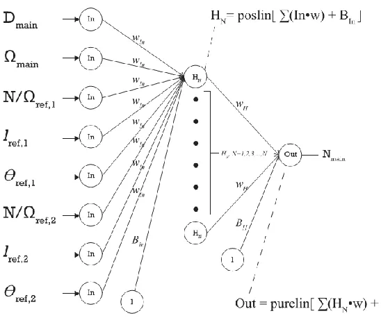
λ is called the regularization parameter which needs to be tuned as a hyper-parameter while w refers to the weight in the network. Therefore, the goal of the training algorithm, PSO, is to minimize the C function. The process of tuning the λ will be discussed later in the model selection section. Meanwhile, the type of ANN used in this research was a fully connected ANN where all hidden nodes are connected evenly to all the input parameters and output. Figure 2 shows the topology of the ANN-PSO models.

Figure 2. Figure shows the topology of ANN-PSO models, poslin and

purelin are the activation functions.

3.4. Model Training, Selection and Testing

The neural network models were trained using the particle swarm optimization method. Five different models were trained: ANN-PSO I, ANN-PSO II, ANN-PSO III, ANN-PSO IV and ANN-PSO V. The objective of each model was to predict the SPT-N value of the borehole corresponding to the name of the model. Therefore, no data from the borehole to be predicted was included in the training set of the model. For example, ANN-PSO I’s objective was to predict Borehole 1’s SPT-N value thus no data from Borehole 1 was used during the training stage. This method was repeated for the other models.

[image:6.595.167.441.322.551.2]

same configuration space as would be spanned by a regular grid. Based on the result of the paper, random search is found to give better models in most cases and required less computational time.

There were three hyper-parameters which needed to be tuned; Number of neurons in the hidden layer (Nh), dynamic range of PSO problem space (Dr) and regularization parameter (λ). Therefore, the best model for each of ANN-PSO I, ANN-PSO II, ANN-PSO III, ANN-PSO IV and ANN-PSO V are the one with the most optimum hyper-parameter value. The most optimum hyper-parameter values are selected based on the model’s performance on the validation set. A total of 100 random search trials were conducted for each model. Then the trial which exhibited the best performance on the validation set was selected as the best model. Each trial was conducted for 500 iterations with a particle swarm size of 150.

After the best models were selected, each model was tested using the testing set. The testing set for each model were divided into 6 set (Test Set A, B, C, D, E and F). They were divided based on the combination of reference borehole used. For example, for ANN-PSO I, Test Set A predicts N-value of BH1 using data from BH2 and BH3 meanwhile Test Set B predicts N-value of BH1 using data from BH3 and BH4. The prediction from Test Set A, B, C, D, E and F are then added together and divided by the size of the sample to get the average prediction of BH1. The performance metric used for the testing stage were the coefficient of determination, R2 _{and mean absolute error, MAE.}

MAE was calculated using equation 7.

) (e_t mean

MAE  (7)

Then, R2 was calculated using equation 8 [17].

2

2 2

2 2

2 )

) ) ) ( )(

( (

) )( ( ) ( (



















 

y y

n x x

n

y x xy

n

R (8)

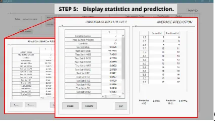
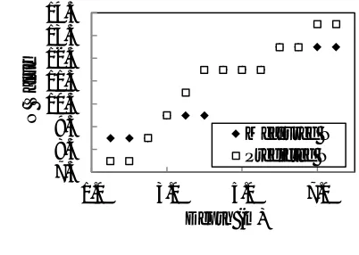
In theory, an R2 close to 1 indicates good performance while for MAE, value closer to zero indicates less margin of error. Figure 3, 4, 5, 6, 7, 8 and 9 shows screenshot of the ANN-SPO program.

4. Results and discussion

The performance of the ANN-PSO models in terms of R2 _{from best to worst; ANN-PSO III (0.85),}

ANN-PSO I (0.82), ANN-PSO IV (0.79), ANN-PSO II (0.77) and ANN-PSO V (0.17) meanwhile in terms of MAE from best to worst; PSO III (0.54), PSO I (0.69), PSO IV (1.08), ANN-PSO II (1.38) and ANN-ANN-PSO V (4.62). The probable cause of the poor performance of ANN-ANN-PSO V would also be discussed in later section. The optimum hyper-parameters are shown in Table 2 while the outputs of each ANN model are shown below with their actual measured value in Table 3.

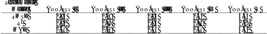
Table 2. ANN-PSO Optimum Hyper-Parameters from the result of random search.

ANN-PSO I ANN-PSO II ANN-PSO III ANN-PSO IV ANN-PSO V

Nh Dr λ Nh Dr λ Nh Dr λ Nh Dr λ Nh Dr Λ

[image:8.595.75.542.131.284.2]

Table 3. ANN-PSO’s output and the corresponding actual measured N value.

Depth (m)

ANN-PSO I ANN-PSO II ANN-PSO III ANN-PSO IV ANN-PSO V

Actual N

Predicted N

Actual N

Predicted N

Actual N

Predicted N

Actual N

Predicted-N

Actual N

Predicted N

1.5 10 9 5 6 9 8 9 11 10 6

2.0 10 9 5 6 9 8 9 11 10 7

2.5 10 9 5 6 9 9 9 11 10 7

3.0 9 9 10 8 10 10 14 12 16 8

3.5 9 10 10 8 10 11 14 12 16 8

4.0 9 10 10 9 10 12 14 13 16 9

4.5 12 11 9 8 12 12 14 13 18 9

5.0 12 11 9 8 12 12 14 13 18 10

5.5 12 12 9 8 12 12 14 14 18 12

6.0 13 13 10 9 13 13 16 14 14 13

6.5 13 13 10 10 13 13 16 15 14 13

7.0 13 14 10 11 13 14 16 15 14 14

7.5 15 14 12 11 13 14 16 15 16 14

4.1. ANN-PSO’s Graphical User Interface

[image:8.595.151.445.396.563.2]

ANN-PSO was the program developed as a result of this research. The ANN-PSO program receives input data from Excel files and outputs the estimated N value inside MATLAB’s workspace. There are five modes of PSO which is PSO I, PSO II, PSO III, PSO IV and ANN-PSO V. Three groups of settings that need to be specified by the user are hyper-parameter range, fixed parameter and the random trial setting. ANN-PSO also displays the visualization of the particle swarm movement in a 3-dimensional space.

Figure 3. Main interface of ANN-PSO program

[image:8.595.77.289.611.736.2] [image:8.595.317.529.614.733.2]

[image:9.595.317.528.120.237.2] [image:9.595.77.292.122.237.2]

Figure 6. ANN-PSO settings. Figure 7. Manual search or random search.

Figure 8. ANN-PSO’s diplays the output. Figure 9. ANN-PSO’s swarm movement (150 particles)

4.2. Coefficient of Determination, R2

[image:9.595.323.516.284.461.2] [image:9.595.78.291.314.434.2]

[image:10.595.98.303.128.261.2] [image:10.595.344.534.128.260.2]

Figure 10. Observed N vs. Estimated N (ANN-PSO I).

[image:10.595.344.536.362.496.2]

Figure 11. Observed N vs. Estimated N (ANN-PSO II).

Figure 12. Observed N vs. Estimated N (ANN-PSO III).

Figure 13. Observed N vs. Estimated N (ANN-PSO IV).

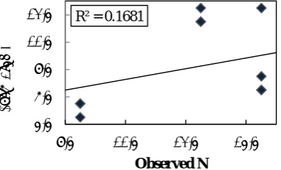
Figure 14. Observed N vs. Estimated N (ANN-PSO V).

R² = 0.8233

8 10 12 14 16

8 10 12 14 16

Es ti m ate d N Observed N

R² = 0.773

4 6 8 10 12

4 6 8 10 12

Es ti m ate d N Observed N

R² = 0.8493

8 9 10 11 12 13 14

8.5 9.5 10.5 11.5 12.5 13.5

Es ti m ate d N Observed N

R² = 0.7926

10.5 11.5 12.5 13.5 14.5 15.5

8.5 10.5 12.5 14.5 16.5

Es ti m ate d N Observed N

R² = 0.1681

5.5 7.5 9.5 11.5 13.5

9.5 11.5 13.5 15.5

[image:10.595.94.308.364.508.2] [image:10.595.103.301.604.723.2]

4.3. Mean Absolute Error

Meanwhile, in terms of MAE, ANN-PSO I, ANN-PSO II, ANN-PSO III, ANN-PSO IV, and ANN-PSO V scored 0.69, 1.08, 0.54, 1.38 and 4.62 respectively. With MAE values below 1 for ANN-PSO I and ANN-PSO III, it can be said that these two models possess good margin of error capable of predicting N-value with good confidence. Since N-values are typically used only as a rough measure of density of soil, ANN-PSO II and ANN-PSO IV are deemed to be within acceptable margin of error. However, as with the performance of ANN-PSO V on R2, ANNPSO V’s performance based on MAE is poor and indicates problems with the training sets. Figure 15, 16, 17, 18 and 19 shows the comparison between measured N and predicted N for each model.

Figure 15. Observed N and Estimated N at varying depth (ANN-PSO I).

Figure 16. Observed N and Estimated N at varying depth (ANN-PSO II).

Figure 17. Observed N and Estimated N at varying depth (ANN-PSO III).

Figure 18. Observed N and Estimated N at varying depth (ANN-PSO IV).

8 10 12 14 16

1.0 3.0 5.0 7.0

N V al u e Depth (m) Measured N Predicted N 4.5 6.5 8.5 10.5 12.5

1.0 3.0 5.0 7.0

N V al u e Depth (m) Measured N Predicted N 7.5 8.5 9.5 10.5 11.5 12.5 13.5 14.5

1.0 3.0 5.0 7.0

N V al u e Depth (m) Measured N Predicted N 8.5 10.5 12.5 14.5 16.5

1.0 3.0 5.0 7.0

[image:11.595.88.280.243.374.2] [image:11.595.333.520.247.375.2] [image:11.595.78.279.489.632.2] [image:11.595.320.517.489.634.2]

Figure 19. Observed N and Estimated N at varying depth (ANN-PSO V).

4.4. Summary of ANN-PSO Models’ Performance

[image:12.595.88.302.123.272.2]

A summary of statistical performance of all five ANN-PSO models can be seen in Table 4.

Table 4. Statistical Performance of ANN-PSO Models.

Performance

Metric ANN-PSO I ANN-PSO II ANN-PSO III ANN-PSO IV ANN-PSO V

RMSE 0.83 1.18 0.83 1.52 5.53

R2 _{0.82 0.77 0.85 0.79 0.17}

MAE 0.69 1.08 0.54 1.38 4.62

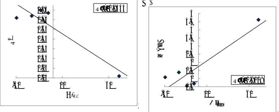
4.5. ANN-PSO V’’s Analysis

In order to investigate why ANN-PSO V’s performance is relatively poor compared to the other models, an analysis of the training set and testing set of all the models were conducted. During the analysis, the difference between the mean of lref input parameter in the training and the lref input parameters in the

testing set,



l

ref , was found to be negatively correlated with the R2 value and positively correlated with the MAE value. This means that a high



l

ref value, which the case for ANN-PSO V, would cause low R2 value and higher MAE value.



l

refwas calculated by averaging all the lref input value in the

training set to get

l

ref,Train and the same was done in the testing set to get

l

ref,Test. Then,



l

ref value was calculated by using equation 9.

Train ref Test ref

ref

l

l

l



,



,



(9)

Table 5.



l

ref , R2 and MAE for each Model.

Model 𝛥 𝑙̅𝑟𝑒𝑓 R2 MAE

ANN-PSO I -5.17 0.82 0.69 ANN-PSO II -39.33 0.77 1.08 ANN-PSO III -13.5 0.85 0.54 ANN-PSO IV -23.08 0.79 1.38 ANN-PSO V 71.08 0.17 4.62

5.5

7.5 9.5 11.5 13.5 15.5

1.0 3.0 5.0 7.0

S

P

T

-N

Depth (m)

[image:12.595.73.521.364.422.2] [image:12.595.110.486.642.715.2]

From Table 5, it is quite clear that



l

ref for ANN-PSO V is an outlier compared to the other model. The lowest



l

ref value is for ANN-PSO I with a value of -5.17 while the highest



l

ref is for ANN-PSO V with a value of 71.08. The relationship between



l

ref and R2is shown in Figure 20 meanwhile the relationship between



l

ref and MAE is shown in Figure 21.

-Figure 20. Correlation between



l

ref and R2 Figure 21. Correlation between



l

ref and MAE

4.6. Optimum Swarm Size

[image:13.595.76.526.215.396.2]

In order to investigate the optimum number of particles in the swarm, a trial run was conducted using ANN-PSO III. The hyper-parameters settings were set as follows; Hn = 2, Dr = 4 and λ = 3 for all swarm size. The PSO algorithm was set to run for 250 iterations using swarm size of 50, 100, 150 and 200 particles. Figure 22 shows the comparison between the convergences of different swarm sizes.

Figure 22. Convergence of different Swarm Sizes.

R² = 0.8543

0.15 0.25 0.35 0.45 0.55 0.65 0.75 0.85

-40 10 60

R

2

Δ lref

R² = 0.8109 0.5

1 1.5 2 2.5 3 3.5 4 4.5 5

-40 10 60

M

A

E

Δ lref

0 10 20 30 40 50 60 70 80

0 50 100 150 200 250

C

o

st

Iterations

[image:13.595.92.510.547.696.2]

From Figure 22, we can see that, the optimum swarm size for this problem is 150 particles. A swarm size of 150 was able to achieve the best minimum value and was able to converge with lesser amount of iterations. It can also be seen that larger swarm size was able to achieve better Cost value in earlier part of the iterations. Furthermore, all the swarm sizes have shown the ability to converge at around 200 iterations although with different minimum Cost value.

5. Conclusions

This research proposes a resource efficient method which combines the use of both SPT and Soil Resistivity Survey using ANN-PSO prediction modeling technique. Five different ANN-PSO models were coded using MATLAB namely ANN-PSO I, ANN-PSO II, ANN-PSO III, ANN-PSO IV and ANN-PSO V with the purpose of each model is to predict BH1, BH2, BH3, BH4 and BH5 respectively. The analysis of the performance shows that ANN-PSO III was the best model while the worst model was ANN-PSO V. Through the analysis of the training set and testing set input parameter, it was shown

that it is possible to predict the performance of ANN-PSO models by calculating



l

ref .

ANN and PSO were found to be particularly useful for solving regression problem. Using an ANN trained by PSO, the ANN was able to estimate N value using resistivity value with acceptable accuracy. The ANN-PSO model developed was able to minimize MSE value over 500 iterations. In the field of civil engineering, there is no shortage of regression problems for researchers and ANN can be used as an alternative to statistical techniques such as Linear Regression and Ordinary Least Squares Regression. The main advantage ANN have over the statistical technique are that researchers do not need to make any assumption (distributional and form) regarding the model whereas ANN is a black box which excels in approximating any type of function. Furthermore, the optimum swarm size for this regression problem was found to be 150 particles and the algorithm converges at around 250 iterations.

Utilizing MATLAB’s GUI feature, a program named ANN-PSO was developed. ANN-PSO is an ANN trained using PSO designed to estimate N-value using Resistivity value. The input of the ANN are Dmain, Ωmain, N/Ωref,1, lref,1, Ɵref,1, N/Ωref,2, lref,2 and Ɵref,2 and the ANN output is Nmain. The program is able to output N value and also provides the user with statistical parameters for analysis purposes.

The method proposed was shown to be able to estimate new borehole DATA using existing borehole data and resistivity data. Aside from ANN-PSO V’s poor performances due to inadequate training set, encouraging result were obtained from the four successful ANN-PSO models, which shows that PSO algorithm is capable of training a Neural Network with exceptional result. The best performance of the ANN-PSO algorithm comes through ANN-PSO III, with an R2 _{= 0.8493 and MAE = 0.54, which is an}

exceptional result in terms of accuracy. Meanwhile, it has been shown that by calculating



l

ref , we can predict whether ANN-PSO is capable of generating estimated N value with an acceptable accuracy or not.

Acknowledgement

The work presented in this paper was developed with the financial support of Universiti Teknologi Malaysia under the Grant Number: R.J130000.7822.4J222 and Q.J130000.2622.15J26.

References

[1] Samouelian, A., Cousin, I., Tabbagh, A., Bruand, A., & Richard, G. 2005. Electrical resistivity survey in soil science: A review. Soil and Tillage Research, 83(2), 173–193. [2] Hatta, K. A., & Syed Osman, S. B. A. 2015. Correlation of Electrical Resistivity and

N Value from Standard Penetration Test (SPT) of Sandy Soil. Applied Mechanics and Materials, 785, 702–706.

[3] Mahmoud, M. A. A. N. 2013. Reliability of Using Standard Penetration Test (SPT) in Predicting Properties of Silty Clay with Sand Soil. International Journal of Civil and

[4] Tonnizam Mohamad, E., Jahed Armaghani, D., Hasanipanah, M., Murlidhar, B. R., & Alel, M. N. A. 2016. Estimation of air-overpressure produced by blasting operation through a neuro-genetic technique. Environmental Earth Sciences,75(2), 1–15.

[5] Flood, I., & Kartam, N. 1994. Neural Networks in Civil Engineering. Principles and

Understanding,33, 669–682.

[6] Elarabi, H., & Abdelgalil, S. A. 2014. Application of artificial neural network for prediction of`Sudan soil profile, American Journal of Engineering, Technology and Society, 1(2), 7–10. [7] Erzin, Y., & Gul, T. O. 2014. The use of neural networks for the prediction of the settlement

of one-way footings on cohesionless soils based on standard penetration test. Neural

Computing and Applications, 24(3), 891–900.

[8] Majdi, A., & Rezaei, M. 2013. Prediction of Unconfined Compressive Strength of Rock surrounding a Roadway using Artificial Neural Network. Neural Computing and

Applications, 23(2), 381–389.

[9] Kuok, K. K., Harun, S., & Shamsuddin, S. M. 2010. Particle Swarm Optimization Feedforward Neural Network for Modeling Runoff. International Journal of Environment

Science & Technology, 7(1), 67–78.

[10] Garro, B. A., & Vázquez, R. A. 2015. Designing Artificial Neural Networks using Particle Swarm Optimization Algorithms. Computational Intelligence and Neuroscience, 20.

[11] Mohammadi, N., & Mirabedini, S. J. 2014. Comparison of Particle Swarm Optimization and Backpropagation Algorithms for Training Feedforward Neural Network. Journal of

Mathematics andComputer Science, 12, 113–123.

[12] Eberhart, R., & Shi, Y. 2001. Tracking and Optimizing Dynamic Systems with Particle Swarms. Proceedings of the 2001 Congress on Evolutionary Computation, 1, 94–100. [13] Hagan, M. T., Demuth, H. B., & Beale, M. H. 1995. Neural Network Design. Boston

Massachusetts PWS, 2, 734.

[14] Huber, R., & Mayer, H. A. 1996. On the Role of Regularization Parameters in Fitness Functions for Evolutionary Designed Artificial Neural Networks. In Proceeding of World

Congress on Neural Networks (pp. 1063–1066).

[15] Kriesel, D. 2005. A Brief Introduction to Neural Networks. 6080(94)90051-5

[16] Bergstra, J., & Yoshua, B. 2012. Random Search for Hyper-Parameter Optimization. Journal

of Machine Learning Research, 13, 281–305.

[17] Mukaka, M. M. 2012. A guide to appropriate use of correlation coefficient in medical research.