Algorithm of construction of Optimum Portfolio of stocks using Genetic Algorithm

(1)

Algorithm of construction of Optimum

Portfolio of stocks using Genetic

Algorithm

Sinha, Pankaj and Chandwani, Abhishek and Sinha, Tanmay

Faculty of Management Studies, University of Delhi

10 July 2013

(2)

Sinha P.,Chandwani A., Sinha T. Page 1

Algorithm of construction of Optimum Portfolio of

stocks using Genetic Algorithm

Pankaj Sinha

Faculty of Management Studies, University of Delhi

Abhishek Chandwani

Indian Institute of Technology, Kharagpur

Tanmay Sinha

Jaypee Institute of Technology, Noida

Abstract:

The objective of this paper is to develop an algorithm to create an Optimum Portfolio from a large pool of stocks listed in a single market index SPX 500 Index: USA (for example) using Genetic Algorithm. The algorithm selects stocks on the basis of a priority index function designed on company fundamentals, and then genetically assigns optimum weights to the selected stocks by finding a genetically suitable combination of return and risk on the basis of historical data. The effect of genetic evolution on portfolio optimization has been demonstrated by developing a MATLAB code to implement the genetic application of reproduction, crossover and mutation operators. The effectiveness of the obtained portfolio has been successfully tested by running its performance over a six month holding period. It is found that genetic algorithm is successful in providing the optimum weights to stocks which were initially screened through a predetermined priority index function. The constructed portfolio beats the market for the considered holding period by a significant margin.

(3)

1. Introduction:

The process of genetic evolution which has been verified by the laws of nature since the beginning of earth is proven to be the most intricate and beautiful optimization technique. The key elements of Genetic Algorithm are:

i) Creation of Chromosomes ii) Initiating Parent Species iii) Creation of Initial Population

iv) Reproduction Pool on the basis of Fitness Selection v) Genetic Operators: Crossover

vi) Mutation Operation

This study applies the very concepts of above genetic evolution in constructing an optimum portfolio of stocks selected from a large pool of stocks listed in the single market index. We have put in our utmost efforts to contribute significant analytical conclusion to the application of genetic algorithm on the issue of optimization of weights of stocks selected in the portfolio. The algorithm for portfolio construction involves two stages - selection of stocks by using a priority index function and optimization of the weights of the selected stocks The process initially selects stocks for the portfolio on the basis of fundamentals of the company using a priority index function and then it optimizes the weights of the selected stocks by a genetic approach, where the selected stocks were allowed to genetically evolve towards the fittest population taking into account both risk and return of stocks. A systematic and computational mode of Darwinian evolution has been applied in this research paper. The optimization of stocks will be adjusted as per the stocks undergo a genetic evolution through the process of reproduction and mating using crossover and mutation.

1.1Genetic Algorithm

The entire process of optimization by Genetic Algorithm is explained in the following steps:

i) The process was initiated by starting a random solution called ‘Population’ which consists of chromosomes.

ii) Each chromosome represents a solution of the problem with genes representing the weight given to each selected stock.

(4)

Sinha P.,Chandwani A., Sinha T. Page 3 iv) These chromosomes are then made to evolve genetically through iterations

giving rise to newer populations.

v) We compare the fitness values of evolving chromosomes with the existing chromosomes, after each iteration. The objective function used to calculate fitness is described in the following section.

vi) In this study we evaluate the objective function over a large population size such that the objective function attains the maximum possible value.

vii) After all the iterations are over, we calculate the fitness value of each of the chromosomes and select the chromosome which attains the maximum fitness value , in accordance with Darwin’s (1859)theory of survival of the fittest.

viii) This selected chromosome shall represent the optimization of the weights of the stocks giving us genetically suitable return and risk.

ix) This genetic procedure is designed to maximize the fitness value under the constraint that the sum of the weights is 1 and that all the weights are less than 1 and greater than zero.

(5)

[image:5.595.70.525.76.610.2]

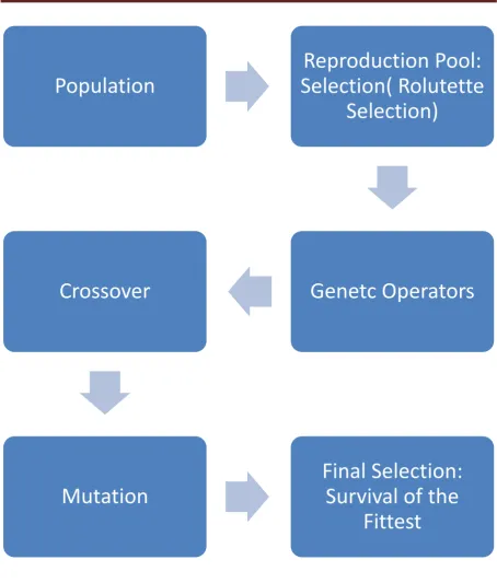
Sinha P.,Chandwani A., Sinha T. Page 4 Figure 1: Genetic Evolution Mechanism

Population

Reproduction Pool:

Selection( Rolutette

Selection)

Genetc Operators

Crossover

Mutation

Final Selection:

Survival of the

(6)

Sinha P.,Chandwani A., Sinha T. Page 5 The following various functions are used in the algorithm:

i) Objective Function

Maximize Risk and simultaneously Minimize Risk Portfolio Return= Σ wiri

Portfolio Variance ( 2p )= Σwi2 i2+ Σ Σ2*wi*wj*cov(I,j)) Such that Σwi= 1

Where wi= weight of ith stock Ri= average return of ith stock

f( chromosome)= Portfolio Return /Portfolio Standard Deviation

Where:

wi= weight of ith stock Wj=weight of jth stock

f(chromosome)=fitness value of the chromosome Cov(I,j)= Covariance of Returns between the ith and jth stocks

ii) Evaluation Function

This function shall be used to create the reproduction pool from the parent population. The evaluation function is similar to the probability which decides the fitness of the species. It is the ratio of the fitness value of the ith chromosome to the sum of fitness values of all the chromosomes.

f(evaluation i)=f(chromosome i)/ Σ f(chromosome i)

1.2 Population Initiation

i) A population shall consist of chromosomes which shall be made up of genes. A gene is representative of values which shall return weights of the selected stocks.

(7)

Sinha P.,Chandwani A., Sinha T. Page 6 iii) These obtained random values (Vi) are now used to calculate weights (wi) of the

selected stocks by calculating Vi/(Σ Vi).These weights are the stock wise percentages of the total investment which the portfolio manager shall recommend to the user.

iv) A parent population of 10 random chromosomes representing 10 random initial solutions to the objective function is created.

1.3 Reproduction Pool: The method of selection

i) The method shall decide the reproduction pool that is the chromosomes which shall undergo mating. There are several available techniques like: Tournament Selection, Roulette Wheel Selection, Stochastic Based Selection and Reward Based Selection. In this paper we have used the Roulette Wheel Selection (also known as the Fitness Proportionate Selection) in order to select the species on the basis of their fitness values mainly.

Roulette Selection:

ii) Each chromosome is evaluated on the basis of the fitness function (as mentioned above).

iii) A random number (ri) is generated from normal distribution and is compared with the chromosome’s cumulative probability. The chromosome i having cumulative probability such that p(i-1)<ri.< pi is selected into the reproduction pool.

iv) The reproduction pool shall consist of species which have been selected by the Roulette Selection Method defined above.

1.4 Genetic Mating

Crossover:

Crossover can be performed by a variety of methods:

a) Single Point Crossover b) Two Point Crossover c) Uniform Crossover d) Heuristic Crossover

(8)

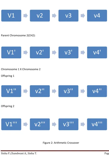
Sinha P.,Chandwani A., Sinha T. Page 7 Offspring 1= a*CH1+ (1-a)*CH2

Offspring 2= (1-a)*CH2+ a*CH2

Where a=Any random number belonging to (0,1)

Parent Chromosome 1 (CH1):

Parent Chromosome 2(CH2):

Chromosome 1 X Chromosome 2

Offspring 1

[image:8.595.68.511.166.794.2]

Offspring 2

Figure 2: Arithmetic Crossover

V1

v2

v3

v4

V1'

v2'

v3'

v4'

V1''

v2''

v3''

v4''

(9)

Sinha P.,Chandwani A., Sinha T. Page 8 The new values(v’’ and v’’’) can be calculated by the formula given above, where in a is random number between 0 and 1.The Figure above represents arithmetic point crossover and describes how two parent chromosomes mate by crossover to give the two off springs. Each of these values shall now give different weights to the stocks 1,2,3..n, Hence allowing genetic evolution by crossover.

Where:

V’’=a*V + (1-a)*v’ V’’’= (1-a)*v + a*v’

Mutation:

Parent Chromosome

Mutation Point 1 Mutation Point 2

Offspring

Figure3 : Mutation

V1

v2

v3

v4

(10)

Sinha P.,Chandwani A., Sinha T. Page 9 The gene at the mutation point 1 shall move to the mutation point 2 while the others shall

shift a position each towards the initial position of mutation point 1.

1.5 Decision of Crossover versus Mutation

This is a question which has seldom been addressed when dealing with a large data set, the problem of how to understand which species shall undergo crossover and which shall decide to mutate.

We considered the following points before deciding on the approach to tackle this issue:

i) The solution depends on the nature of problem to a large extent. The solution should be oriented in such a way that the genesis contributes to evolution of the species selecting the fittest species which is decided on the basis of fitness function.

ii) Crossover is a primarily explorative procedure, it accommodates the features of both the parents and creates a chromosome somewhere in between the parents.

iii) Mutation is exploitative; it only creates a slight diversion with the parent and hence alters the feature locally.

iv) Only crossover can combine information from two parents where as mutation shall introduce new information into the offspring. Hence we need a lucky mutation for a perfect genesis.

v) The paper has found on the basis of probabilistic approach that a mutation probability of Pm=0.4 and a crossover probability of Pc=0.6 shall yield the optimum solution.

vi) In case of identical chromosomes being selected in the reproduction pool, the stocks shall mutate in order to obtain a genetic advantage for the next

population.

(11)

2. Literature Review

Markovitz (1952), the father of Modern Portfolio theory, has established the role of combining different assets to minimize risk of the portfolio constructed via his publication. We have incorporated his conclusions in our research by keeping diversity a factor while constructing the portfolio. We achieved this by dividing the initial pool of stocks into sectors allowing the representation of each sector in the portfolio thus reducing the risk.

Melanie M. (1998) and M.Gen and R. Cheng (1997) explains the process of genetic algorithm in detail. They have presented various mathematical models for applying evolutionary genetic technique.

Lin and Gen (2007) stresses on the importance of taking risk as well as return into consideration while portfolio selection. The paper suggested that the multi stage genetic algorithm can be used for the portfolio optimization. Pereira (2000) has suggested that Genetic Algorithms are a valid approach to optimization problems in finance. Yang (2006) advocates that Genetic Algorithms can be used to improve the efficiency of the portfolio. Bakhtyar et al (2012) discussed that the choice of crossover and mutation influence the Genetic Algorithm performance. Seflane and Benbouziane(2012) shows that arithmetic crossover is genetically better than single point and two point crossover using an example of five stocks, while considering both return and risk in the objective function.

Sinha and Goyal (2012) develops an algorithm for the portfolio construction from a large pool of stocks listed in a single market index SP CNX 500 using MATLAB code.

Motivation

(12)

3. Portfolio Construction: Algorithm

The MATLAB code for the entire process of portfolio construction, as described below, is given in the appendix of this paper.

3.1Stock Selection Procedure:

1. Diversification of Portfolio

The most vital logic behind our portfolio selection is the inclusion of Diversity in our portfolio. We have achieved this by dividing the pool of stocks into sectors namely IT, Telecom, Automobile et al. Now the stocks will be evaluated on the parameters mentioned below using the criteria of maximum and minimum of that sector. This implies that stocks will get selected if their performance score is high in that sector, and thus only best performers from each sector would comprise of our portfolio resulting in a diversified portfolio.

2. Parameters for Selection

The fundamental factors are those which shall allow the user to construct a portfolio based on business performance principle rather than focusing merely on market sentiments. The following factors are essential for determining the stocks in the final portfolio:

I. Price/Earnings (P/E)

The P/E ratio is an important parameter for understanding the earnings per money invested. A P/E ratio of x shall imply an investment of x units of money for unity profit. Generally, an investor shall prefer to choose stocks which have a lower P/E ratio.

II. Earnings/Share (EPS ratio)

Earnings/Share is defined as the portion of company’s profit allotted to each outstanding share of common stock. From an investor’s perspective, a higher EPS is desirable.

III. Wealth Creation

(13)

IV. Undervaluation

Undervaluation is defined as the situation when the stocks of the company are priced such that the market price is lower than the fair price. An investor shall always look to ‘pick up’ undervalued stocks. This is measured by the Market Capitalization to Revenue ratio. If the value of this ratio is less than 1, the stock is considered to be undervalued.

V. (Price is to Earning) / Growth ( PEG ratio)

We have used this parameter to represent a significant comparison between companies having different Price/Earnings Ratios and Growth Percentages. An investor shall always want to invest into businesses having lower PEG values.

The stocks are selected on the basis of their performance in all these parameters on the basis of historical data. The priority function is such designed that stocks having highest score shall be selected into the pool of stocks comprising the portfolio.

Calculation of Priority Index

The Priority Index Function uses the factors mentioned above as the benchmark, and the stocks are ranked on the basis of their cumulative scores as generated by the Priority Index Function. Equities are ranked and allotted a score as per linear interpolation which can be expressed as follows:

Sij=100(Xij-Max)/ (Min-Max)

Where:

Sij=Score of ith stock on jth parameter Xij=Functional Value of ith stock on jth function Min=Minimum Value of ith stock on jth function Max=Maximum value of ith stock on jth function

The formula for values whose minimum is desired is :

Sij=100(Xij-Min)/ (Max-Min)

(14)

Sinha P.,Chandwani A., Sinha T. Page 13 PIi=Σ Sij

The stock selection is based on the Priority Index (PIi) and the algorithm shall create the portfolio from only those stocks which have a Priority Index greater than 3.8 on a 5 point scale.

3.2Portfolio Optimization

i) The stocks selected on the basis of Priority Index are added to the

portfolio and their weights are operated genetically for optimization. The selected stocks comprise of the genes of a chromosome.

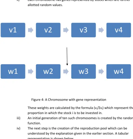
[image:14.595.71.509.255.712.2]

ii) Each chromosome has genes represented by stocks which are further allotted random values.

Figure 4: A Chromosome with gene representation

These weights are calculated by the formula (vi/Σvi) which represent the proportion in which the stock i is to be invested in.

iii) An initial generation of ten such chromosomes is created by the random function.

iv) The next step is the creation of the reproduction pool which can be understood by the explanation given in the earlier section. A tabular representation is shown below.

v1

v2

v3

v4

(15)

Sinha P.,Chandwani A., Sinha T. Page 14 Chromosome(CH) Fitness

Value

Evaluation Function

Cumulative Probability

Random # generated

Chromosome (CH) selected

# of copies of CH received

CH1 1.79 0.22 0.22 0.36 CH2 1

CH2 1.95 0.24 0.46 0.16 CH1 1

CH3 2.10 0.26 0.72 0.57 CH3 2

[image:15.595.71.511.270.773.2]

Ch4 1.87 0.28 1.00 0.63 CH3 0

Table 1: Generation of Reproduction Pool

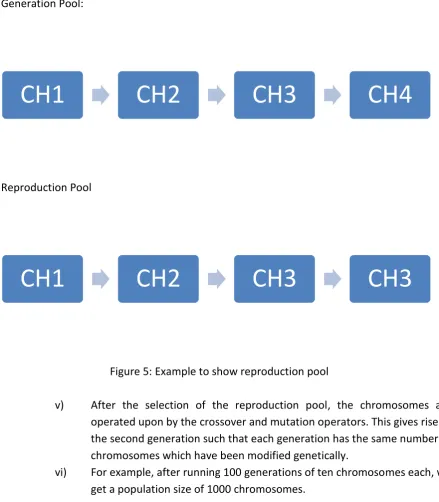
The reproduction pool shall now consist of the chromosomes: CH1, CH2, CH3, and CH3

Generation Pool:

Reproduction Pool

Figure 5: Example to show reproduction pool

v) After the selection of the reproduction pool, the chromosomes are operated upon by the crossover and mutation operators. This gives rise to the second generation such that each generation has the same number of chromosomes which have been modified genetically.

vi) For example, after running 100 generations of ten chromosomes each, we get a population size of 1000 chromosomes.

CH1

CH2

CH3

CH4

(16)

Sinha P.,Chandwani A., Sinha T. Page 15 vii) The chromosome with the best fitness value is selected and the

composition shall be the solution to our portfolio optimization problem.

4. Applied Example of Genetic Algorithm on SP 500 Index: US

Input:

The input shall consist of the stocks from SP 500 Index: US comprising of the daily closing prices, EPS Ratios, PEG Values, Weighted Average Cost of Capital, Market

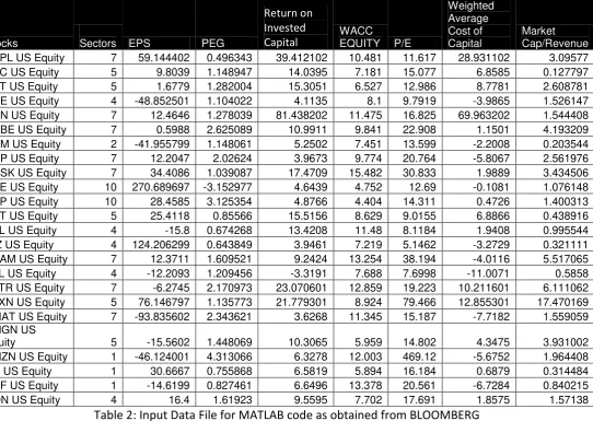
Capitalization/Revenue and Return on Invested Capital in the US Market from the duration December 2011 to December 2012.The input was taken from Bloomberg. The data should be divided sector wise as shown in the column ‘Sectors’ of the Table 2.

[image:16.595.35.578.323.708.2]

A sample input data file obtained from BLOOMBERG is shown as below.

Table 2: Input Data File for MATLAB code as obtained from BLOOMBERG

And the data set shall continue in the same order for all the input stocks (SP500 INDEX: US in our study).

Stocks Sectors EPS PEG

Return on Invested Capital

WACC

EQUITY P/E

Weighted Average Cost of Capital

Market Cap/Revenue

AAPL US Equity 7 59.144402 0.496343 39.412102 10.481 11.617 28.931102 3.09577 ABC US Equity 5 9.8039 1.148947 14.0395 7.181 15.077 6.8585 0.127797 ABT US Equity 5 1.6779 1.282004 15.3051 6.527 12.986 8.7781 2.608781 ACE US Equity 4 -48.852501 1.104022 4.1135 8.1 9.7919 -3.9865 1.526147 ACN US Equity 7 12.4646 1.278039 81.438202 11.475 16.825 69.963202 1.544408 ADBE US Equity 7 0.5988 2.625089 10.9911 9.841 22.908 1.1501 4.193209 ADM US Equity 2 -41.955799 1.148061 5.2502 7.451 13.599 -2.2008 0.203544 ADP US Equity 7 12.2047 2.02624 3.9673 9.774 20.764 -5.8067 2.561976 ADSK US Equity 7 34.4086 1.039087 17.4709 15.482 30.833 1.9889 3.434506 AEE US Equity 10 270.689697 -3.152977 4.6439 4.752 12.69 -0.1081 1.076148 AEP US Equity 10 28.4585 3.125354 4.8766 4.404 14.311 0.4726 1.400313 AET US Equity 5 25.4118 0.85566 15.5156 8.629 9.0155 6.8866 0.438916 AFL US Equity 4 -15.8 0.674268 13.4208 11.48 8.1184 1.9408 0.995544 AIZ US Equity 4 124.206299 0.643849 3.9461 7.219 5.1462 -3.2729 0.321111 AKAM US Equity 7 12.3711 1.609521 9.2424 13.254 38.194 -4.0116 5.517065 ALL US Equity 4 -12.2093 1.209456 -3.3191 7.688 7.6998 -11.0071 0.5858 ALTR US Equity 7 -6.2745 2.170973 23.070601 12.859 19.223 10.211601 6.111062 ALXN US Equity 5 76.146797 1.135773 21.779301 8.924 79.466 12.855301 17.470169 AMAT US Equity 7 -93.835602 2.343621 3.6268 11.345 15.187 -7.7182 1.559059 AMGN US

(17)

Sinha P.,Chandwani A., Sinha T. Page 16 A second input file is a column of the daily market returns for the same duration for the SP 500 Index: US. It is taken as the return of the market portfolio for the calculation of raw Beta of each stock of the index. Adjusted Beta is calculated by using the following relation:

Adjusted Beta=0.67*Raw Beta + 0.33*1

Output:

The portfolio constructed for a threshold of 3.8 on a 5 point scale is shown in the Table 3 below along with the performance analytics. This threshold value has given us a portfolio of 25 stocks selected by the Priority Index Function and Optimized by Genetic Algorithm. The lower the threshold, the higher will be the number of stocks in the portfolio and vice versa.

Equity

%Annual Return

[image:17.595.222.375.287.733.2]

'ADBE US Equity' 6.435194 'AKAM US Equity' 3.14256 'AMZN US Equity' 2.841326 'AVB US Equity' 1.456976 'BEAM US Equity' 11.7248 'BXP US Equity' 1.237292 'CCL US Equity' 4.894944 'CTL US Equity' 4.456662 'EFX US Equity' 3.865197 'EXPE US Equity' 5.850266 'GAS US Equity' 5.276695 'HCN US Equity' 3.299015 'JNPR US Equity' 3.874859 'KIM US Equity' 3.078482 'KO US Equity' 2.502491 'LRCX US Equity' 2.624299 'NBL US Equity' 0.398242 'NTRS US Equity' 2.002546 'PKI US Equity' 8.936224 'PNR US Equity' 4.292124 'PXD US Equity' 4.428024 'RHT US Equity' 2.723802 'RRC US Equity' 2.623591 'SRCL US Equity' 5.10981 'URBN US Equity' 2.924574

(18)

5. Analysis of Portfolio:

We shall now analyze the constructed portfolio on the basis of the following parameters:

i) Average Annual return

The average annual return is calculated from the average daily return as per the following formula:

AAR= (1+ADR)252 -1

This shall give us the annual average return for the portfolio allowing the investor to make a decision.

The AAR of the portfolio is 26.01% on the basis of the historical data (Dec’ 11 to Dec’ 12).

ii) Beta of Portfolio ( p)

The Beta of Portfolio shall be an indicator of the correlated volatility of the asset in relation with the volatility of the index on which the stocks are benchmarked. The Beta of Portfolio is 0.87 which is less than beta of the market portfolio.

iii) Treynor’s Ratio

The return which would be earned in excess as compared to a risk free environment is referred to as the Treynor’s Ratio. This shall be analyzed for the above portfolio.

Treynor’s Ratio=Excess Return/Beta The Treynor’s Ratio is 0.2976.

iv) Jenesson’s Alpha

Jenesson’s Alpha is calculated by the following formula:

= (Rp - Rf) - p (Rm - Rf)

It is used as an indicator to determine the unusual return on the portfolio as compared to the return on the market indicating the effectiveness of the selection and optimization of the portfolio algorithm.

Jenesson’s Alpha of the portfolio constructed is 14.56% which indicates that the portfolio constructed by the algorithm is very effective.

(19)

[image:19.595.73.526.373.678.2]

Sinha P.,Chandwani A., Sinha T. Page 18 Performance Parameters:

Table 5: Performance Parameters of the Optimum Portfolio constructed for the Period (Dec’11 –Dec’12)

Risk Free Return in the US Market is taken as the yield on a US Treasury Bill for 1 year=0.13%

Graphical Analysis:

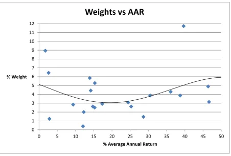
Graph 1. The relation between stock weights assigned and %AAR

The stock weights assigned show an interesting trend, the Genetic Algorithm allotted

weights which were initially decreasing with %AAR and then began increasing after a certain amount. This technique gives insight to the method of optimization of Genetic Algorithm.

0 1 2 3 4 5 6 7 8 9 10 11 12

0 5 10 15 20 25 30 35 40 45 50

% Weight

% Average Annual Return

Weights vs AAR

Priority Index Threshold 3.5/5

No of stocks selected 25

Annual Return of Portfolio

26.01%

Beta of Portfolio 0.87

Treyno's Ratio 0.2976

(20)

Graph 2: Variation of %AAR with Beta Value

The Annual return shows an increasing trend with Beta initially and then begins to decrease. The stocks have been chosen at such a manner that we get values with higher AAR and lower beta values.

Graph 3: Weights versus Beta Value

0.4 20.4 40.4 60.4 80.4 100.4 120.4 140.4

0 1 2

% AAR

Beta of each stock in the portfolio

%AAR vs Beta Value

0 1 2 3 4 5 6 7 8 9 10 11 12

0.6 0.7 0.8 0.9 1 1.1 1.2 1.3 1.4

Weight of stocks in portfolio

Beta Value of stocks in portfolio

(21)

Sinha P.,Chandwani A., Sinha T. Page 20 The weights increase with Beta Value for lower Beta Values but then begin to decrease with higher Beta Values. This shows the optimization technique of the Genetic Algorithm.

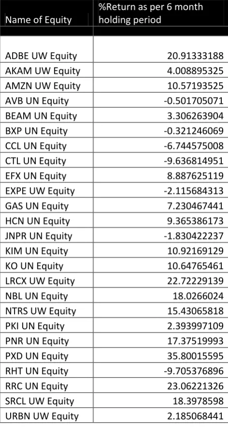
We have analyzed the constructed portfolio on the basis of live data also. Please note that the portfolio was constructed using historical data (December 2011- December 2012). We analyze the constructed portfolio by using the futuristic data (January ’13 – June’13). The analysis shows that the portfolio has performed remarkably with an % AAR as high as 15.98% which was calculated from the six month yield rate of 7.69%. During this period market shows a %AAR if 10.14%, hence the portfolio constructed above using Genetic Algorithm beats the market.

Name of Equity

%Return as per 6 month holding period

ADBE UW Equity 20.91333188

AKAM UW Equity 4.008895325

AMZN UW Equity 10.57193525

AVB UN Equity -0.501705071

BEAM UN Equity 3.306263904

BXP UN Equity -0.321246069

CCL UN Equity -6.744575008

CTL UN Equity -9.636814951

EFX UN Equity 8.887625119

EXPE UW Equity -2.115684313

GAS UN Equity 7.230467441

HCN UN Equity 9.365386173

JNPR UN Equity -1.830422237

KIM UN Equity 10.92169129

KO UN Equity 10.64765461

LRCX UW Equity 22.72229139

NBL UN Equity 18.0266024

NTRS UW Equity 15.43065818

PKI UN Equity 2.393997109

PNR UN Equity 17.37519993

PXD UN Equity 35.80015595

RHT UN Equity -9.705376896

RRC UN Equity 23.06221326

SRCL UW Equity 18.3978598

[image:21.595.174.410.264.707.2]

URBN UW Equity 2.185068441

(22)

6. Conclusion

The study has shown the wide implications of the above two stage process used in portfolio construction:

i) Selection of stocks on the basis of business fundamentals rather than market sentiments is an important lesson for acquiring long term benefits at lower risks. Our portfolio is based on creating a genetically suitable return and risk at the same time. We have successfully reduced the risk by a selection procedure based upon company fundamentals. Thus the portfolio is said to be optimum giving considerable return by taking a calculated risk.

ii) The priority index allows users to select the threshold above which the stocks shall enter the portfolio. Higher the threshold, fewer the stocks and vice versa. This indicates that as the threshold goes up, the decision making becomes stern and we chose stocks which are stronger in business fundamentals. This might compromise on the return but shall give us long term stability.

iii) The research has aptly demonstrated the application of genetic algorithm for optimization of portfolio. This is a novel example of application of Genetic Algorithms in the field of Portfolio optimization in finance.

iv) The portfolio for a threshold of 3.8 on a five point scale gives an annual average return of 15.98% with respect to a risk free return of 0.13%.

(23)

Sinha P.,Chandwani A., Sinha T. Page 22 References

Bakhtyar R., Meraji S.H., Barry D.A., Yeganeah-Bakhtiary A. and Li L. (2012) An application of evolutionary optimization algorithms for determining concentration and velocity profiles in sheet flows and overlying, Journal of Offshore Mechanics and Arctic engineering, Vol. 134, Issue: 2, pp.021802.1-021802.10.

Charles Darwin (1859) On the Origin of Species, John Mayer, London.

Lin C.M., Gen M (2007) An effective Decision based Genetic Algorithm Approach to multi- objective Portfolio Optimization Problem, Applied Mathematical Sciences, Vol 1, Issue: 5, pp. 201-210.

Markowitz H. (1952) Portfolio Selection, Journal of Finance, Vol. 7 , Issue : 1,pp. 77 - 91.

Melanie M. (1998) An Introduction to Genetic Algorithms, MIT Press.

Gen M. and Cheng R. (1997) Genetic Algorithms and engineering Design, John Whiley,New York.

Pereira R. (2000) Genetic Algorithm Optimization for Finance and Investments, MPRA 8610, Univeristy Library of Munich, Germany.

Seflane S. and Benbouziane M. (2012) Portfolio Selection Using Genetic Algorithm, Journal of Applied Finance and Banking ,Vol. 2, Issue : 4, pp. 143-154.

Sinha P. and Goyal L. ( 2012) Algorithm for construction of Portfolio of stocks using Treynor’s Ratio, MPRA Paper 40134, University Library of Munich, Germany.

(24)

Appendix

The MATLAB code for the procedure adopted in the optimum portfolio construction is given below:

%DEFINITION AND NAMES OF VARIABLES USED

%ndata= numerical data related to stock (EPS, PE, PEG, Wealth Creation, MC/RE)

%text= name of all stocks

%value= daily adjusted closing price values of all the stocks %ntms= no of chromosomes to be generated

%l= number of stocks

%m= number of days of which data is available

%value1= daily return of market index(in percentage) %rtrn= daily return of stocks

%marketrtrn= daily return on market

%k= array used for priority function (i.e. to sort and select stocks) %z= array used for counting stocks in each sector

%stk= sorted out stocks by priority function (portfolio)

%stkn= number of stocks selected by priority function (portfolio) %stkrn= return of each stock selected by priority function

%rbs= average daily return of stocks %rb1= average annual return of stocks %rb= arithmatic mean of return

%cv= covariance of return of selected stock

%cvr= covariance of return and market return of each stock %va= variance of market return

%fitness= fitness value of each chromosome %ro= return of each stock in portfolio %rtr1= total return of portfolio

%ann= annual return of the portfolio %betaf= beta of individual stocks %bta= beta of the portfolio

%rpool= reproduction pool containing chromosome details

(weight,value,random value, selected chromosome for crossover or mutation) %chrv= random value for stocks in a chromosome

%chrw= weigth of the stocks in a chromosome %rc= counter used for number of chromosomes %treynors= treynors ratio of portfolio %alpha= alpha of the portfolio

%annmtrn= annual market return

%prfn= threshold value of the Priority Function

%Main Program which is needed to run [Save as: Main.m]

clc;

close all; clear all; prfn=3.8;

ntms=[500 , 1000 , 1500 , 2000 ,2500]; [la,lb]=size(ntms);

for ntimes=1:lb

[ndata, text, alldata] = xlsread('Stock_details.xlsx'); [l,n]=size(ndata);

(25)

v=n; n=n+1;

%adding row number

for i=1:l

ndata(i,n)=i; end

%count of all stocks in each sector

for i=1:10 x=1; for j=1:l

if(ndata(j,1)==i) z(i)=x; x=x+1; end end end %PE k=sortrows(ndata,6); for y=1:10

j(y)=1; end n=n+1; [k,j,z]= sortp(k,l,z,j,n); %PEG k=sortrows(k,3); for y=1:10

j(y)=1; end n=n+1; [k,j,z]= sortp(k,l,z,j,n); %EPS k=sortrows(k,2); for y=1:10

j(y)=z(y); end n=n+1; [k,j,z]= sortm(k,l,z,j,n); %Wealth Creation k=sortrows(k,7); for y=1:10

j(y)=z(y); end n=n+1; [k,j,z]= sortm(k,l,z,j,n); %MC/RE k=sortrows(k,8); for y=1:10

j(y)=1; end

n=n+1;

(26)

n=n+1; for i=1:l k(i,n)=0; for j=v+2:n-1

k(i,n)=k(i,n)+k(i,j); end

end

k=sortrows(k,n);

f=0; for i=1:l

if k(i,n)>=prfn; f=f+1;

for j=1:n

stk(f,j)=k(i,j); end

end

k=sortrows(k,1); stk=sortrows(stk,9); [stkn,stkr]=size(stk);

[value,name] = xlsread('Stock_return.xlsx'); [nn,m]=size(value);

for j=1:nn

rtrn(j,1)=j; end

for i=1:m

rtrn(:,i+1)=value(:,i)/100; rtrn1(:,i)=rtrn(:,i+1); end

[value1] = xlsread('Market_return.xlsx'); value1=transpose(value1);

for i=1:(m)

marketrtrn(i)=value1(i)/100; end

%no of stock screened

y=1;

for i=1:stkn for j=1:nn

if stk(i,9)==rtrn(j,1); txt(y)=text(j); for x=1:m+1

stkr(y,x)=rtrn(j,x); if x>1;

stkrn(y,x-1)=rtrn(j,x); end

end

y=y+1; end

end

(27)

for i=1:stkn

stddv(i)=std(stkrn(i,:)); rbs(i)=1;

for j=1:m

rbs(i)=rbs(i)*(1+stkrn(i,j)); end

rb1(i)=(rbs(i).^(1/252))-1; rb(i)=mean(stkrn(i,:)); end

for i=1:stkn for j=1:stkn cv(i,j)=0; for d=1:252

temp=(stkrn(i,d)-rb(i))*(stkrn(j,d)-rb(j)); cv(i,j)=cv(i,j)+temp;

end

cv(i,j)=cv(i,j)/252; end

end

rbm=mean(marketrtrn); va=var(marketrtrn); for i=1:stkn

cvr(i)=0; for d=1:252

tmp4=(stkrn(i,d)-rb(i)-0.0013)*(marketrtrn(d)-rbm-0.0013); cvr(i)=cvr(i)+tmp4;

end

cvr(i)=cvr(i)/252;

bt1(i)=0.67*(cvr(i)/va)+0.33; end

rc=1;

[rpool,chrv,chrw,fitness,rc] =rpoola(stkn,rb1,cv,rc,stkrn); for i=1:ntms(ntimes)

[rpool,chrv,chrw,fitness,rc]

=rpoolb(rpool,chrv,chrw,fitness,stkn,rb1,cv,rc,stkrn); end

[mxxx,ind]=max(fitness); [mx2,ind1]=max(mxxx);

index=((ind(ind1)-1)*10)+ind1; rtr1(ntimes)=0;

if index >10

ind3=index-mod(index,10); rc=ind3/10;

ind4=mod(index,10); if ind4==0

ind4=10; end

else

rc=1;

ind4=index; end

(28)

bta(ntimes)=0; for i=1:stkn

ro(ntimes,i)=rb1(i)*chrw(rc,ind4,i); rtr1(ntimes)=rtr1(ntimes)+rb1(i)*chrw(rc,ind4,i); betaf(ntimes,i)=bt1(i)*chrw(rc,ind4,i); bta(ntimes)=bta(ntimes)+betaf(ntimes,i); end rtr1(ntimes); bta(ntimes); ann(ntimes)=((1+rtr1(ntimes)).^252-1) treynors(ntimes) =(ann(ntimes))/bta(ntimes); annmtrn=(1+rbm)^252-1; alpha(ntimes)=(ann(ntimes)-0.0013)-bta(ntimes)*(annmtrn-0.0013); end [v1,ind]=max(ann);

xlswrite('output.xlsx',txt(1:stkn)','A1:A10000'); xlswrite('output.xlsx',bt1(1:stkn)','B1:B10000'); xlswrite('output.xlsx',plt(ind,:)','C1:C10000'); xlswrite('output.xlsx',rb1(1:stkn)','D1:D10000'); xlswrite('output.xlsx',alpha(1:lb)','E1:E10000'); xlswrite('output.xlsx',annmtrn','F1');

xlswrite('output.xlsx',ann(ind)','G1');

%sortm function to allot priority grades in ascending order as per the higher value [Save as: sortm.m]

function [k,j,z]= sortm(k,l,z,j,n)

for i=1:l

if k(i,1)==1 ;

k(i,n)=j(1)/z(1); j(1)=j(1)-1;

elseif k(i,1)==2 ;

k(i,n)=j(2)/z(2); j(2)=j(2)-1;

elseif k(i,1)==3 ;

k(i,n)=j(3)/z(3); j(3)=j(3)-1;

elseif k(i,1)==4 ;

k(i,n)=j(4)/z(4); j(4)=j(4)-1;

elseif k(i,1)==5 ;

k(i,n)=j(5)/z(5); j(5)=j(5)-1;

elseif k(i,1)==6 ;

k(i,n)=j(6)/z(6); j(6)=j(6)-1;

elseif k(i,1)==7 ;

(29)

elseif k(i,1)==8 ;

k(i,n)=j(8)/z(8); j(8)=j(8)-1;

elseif k(i,1)==9 ;

k(i,n)=j(9)/z(9); j(9)=j(9)-1;

else k(i,1)=10 ;

k(i,n)=j(10)/z(10); j(10)=j(10)-1; end

end

%sortp function to allot priority grades in descending order as per the higher value [Save as: sortp.m]

function [k,j,z]= sortp(k,l,z,j,n)

for i=1:l

if k(i,1)==1 ;

k(i,n)=j(1)/z(1); j(1)=j(1)+1;

elseif k(i,1)==2 ;

k(i,n)=j(2)/z(2); j(2)=j(2)+1;

elseif k(i,1)==3 ;

k(i,n)=j(3)/z(3); j(3)=j(3)+1;

elseif k(i,1)==4 ;

k(i,n)=j(4)/z(4); j(4)=j(4)+1;

elseif k(i,1)==5 ;

k(i,n)=j(5)/z(5); j(5)=j(5)+1;

elseif k(i,1)==6 ;

k(i,n)=j(6)/z(6); j(6)=j(6)+1;

elseif k(i,1)==7 ;

k(i,n)=j(7)/z(7); j(7)=j(7)+1;

elseif k(i,1)==8 ;

k(i,n)=j(8)/z(8); j(8)=j(8)+1;

elseif k(i,1)==9 ;

(30)

else k(i,1)=10 ;

k(i,n)=j(10)/z(10); j(10)=j(10)+1; end

end

%rpoola function to generate the first reproduction pool [Save as: rpoola.m]

function[rpool,chrv,chrw,fitness,rc] =rpoola(stkn,rb1,cv,rc,stkrn)

for i=1:10 ss=0;

for j=1:stkn

chrv(rc,i,j)=randn(); if chrv(rc,i,j)<0;

chrv(rc,i,j)=chrv(rc,i,j)*(-1); end

ss=ss+chrv(rc,i,j); end

for j=1:stkn

chrw(rc,i,j)=(chrv(rc,i,j)/ss); end

end

for y=1:10 sumchr(y)=0; newv(y)=0;

for i=1:stkn

va1=var(stkrn(i)); for j=1:stkn

sumchr(y)=((sumchr(y)+2*cv(i,j)*chrw(rc,y,i)*chrw(rc,y,j))); newv(y)=newv(y)+rb1(j)*chrw(rc,y,j);

end

sumchr(y)=sumchr(y)+chrw(rc,y,i).^2*va1; end

sumchr(y)=sqrt(sumchr(y));

fitness(rc,y)=newv(y)/sumchr(y);

end

k=y; sum1=0;

for i=1:10

sum1=sum1+fitness(rc,i);

end

sfit(rc)=sum1;

pl=1; rrp=0;

for i=1:10

rpool(rc,i,pl)=i;

(31)

rpool(rc,i,pl+2)=rpool(rc,i,pl+1)/sfit(rc); rrp=rrp+rpool(rc,i,pl+2);

rpool(rc,i,pl+3)=rrp; rpool(rc,i,pl+4)=rand();

end

for i=1:10 j=1; mnx=1;

while(rpool(rc,j,pl+3)<rpool(rc,i,pl+4))

mnx=j; j=j+1; end

rpool(rc,i,pl+5)=mnx;

end

for i=1:10

countrp=histc(rpool(rc,:,6),i); rpool(rc,i,pl+6)=countrp;

if countrp>0

rpool(rc,i,pl+7)=rpool(rc,i,pl+1); else

rpool(rc,i,pl+7)=0; end

end

k=0;

[chrv,fitness,k,stkn,chrw,sumchr,newv,rb1,cv,rpool,pl,rc,yyy] = crossb(chrv,fitness,k,stkn,chrw,sumchr,newv,rb1,cv,rpool,pl,rc);

if yyy>0

end if yyy>0

end

for i=1:10

while rpool(rc,i,8)>0

[chrv,fitness,k,stkn,chrw,sumchr,newv,rb1,cv,rpool,pl,rc] = mutate(chrv,fitness,k,stkn,chrw,sumchr,newv,rb1,cv,rpool,pl,rc); end

end

rc=rc+1;

%crossb function for the crossover between two chromosomes [Save as: crossb.m]

function [chrv,fitness,k,stkn,chrw,sumchr,newv,rb1,cv,rpool,pl,rc,yyy] =

crossb(chrv,fitness,k,stkn,chrw,sumchr,newv,rb1,cv,rpool,pl,rc)

largest = rpool(rc,1,8); x=1;

secondLargest = 0; y=0;

for j=2:10

(32)

if number > largest

secondLargest = largest; largest = number;

y=x; x=j; else

if number > secondLargest secondLargest = number; y=j;

end

yyy=y;

if y>0

rpool(rc,x,7)=rpool(rc,x,7)-1; rpool(rc,y,7)=rpool(rc,y,7)-1; for i=1:10

if rpool(rc,i,7)<1 rpool(rc,i,pl+7)=0; end

end

i=k+1; aa=rand(); for j=1:stkn

chrv(rc+1,i,j)=(1-aa)*chrv(rc,x,j)+(aa*chrv(rc,y,j)); chrv(rc+1,i+1,j)=(aa)*chrv(rc,x,j)+((1-aa)*chrv(rc,y,j)); end

for i=k+1:k+2 ss=0;

for j=1:stkn

ss=ss+chrv(rc+1,i,j); end

for j=1:stkn

chrw(rc+1,i,j)=(chrv(rc+1,i,j)/ss); end

end

for y=k+1:k+2 sumchr(y)=0; newv(y)=0;

for i=1:stkn for j=1:stkn

sumchr(y)=((sumchr(y)+cv(i,j)*chrw(rc+1,y,i)*chrw(rc+1,y,j))); newv(y)=newv(y)+rb1(j)*chrw(rc+1,y,j);

end

fitness(rc+1,y)=newv(y)/sumchr(y); end

k=k+2;

(33)

%mutate function for the mutation of chromosome [Save as: mutate.m]

function [chrv,fitness,k,stkn,chrw,sumchr,newv,rb1,cv,rpool,pl,rc] =

mutate(chrv,fitness,k,stkn,chrw,sumchr,newv,rb1,cv,rpool,pl,rc)

xx=0; i=1;

while i<=10 && xx==0 if rpool(rc,i,7)>0

rpool(rc,i,7)=rpool(rc,i,7)-1; if rpool(rc,i,7)<1

xx=i; end

i=i+1;

end

i=k+1;

for j=1:stkn

chrv(rc+1,i,j)=chrv(rc,xx,j);

end

j1=(17/27)*stkn; j2=1;

while j2<j1 j2=j2+1;

end

j3=(14/27)*stkn; j4=1;

while j4<j3 j4=j4+1;

end

temp=chrv(2,i,j2+1);

for j=j4:j2

temp1(j)=chrv(rc+1,i,j);

end

for j=j4+1:j2+1

chrv(rc+1,i,j)=temp1(j-1);

end

chrv(rc+1,i,13)=temp;

ss=0;

for j=1:stkn

ss=ss+chrv(rc+1,i,j);

end

for j=1:stkn

chrw(rc+1,i,j)=(chrv(rc+1,i,j)/ss);

end

y=k+1;

sumchr(y)=0; newv(y)=0;

for i=1:stkn for j=1:stkn

(34)

newv(y)=newv(y)+rb1(j)*chrw(rc+1,y,j); end

end

fitness(rc+1,y)=newv(y)/sumchr(y); k=k+1;

%rpoolb function to generate the remaining number of reproduction pools [Save as: rpoolb.m]

function[rpool,chrv,chrw,fitness,rc]

=rpoolb(rpool,chrv,chrw,fitness,stkn,rb1,cv,rc,stkrn)

for i=1:10 ss=0;

for j=1:stkn

chrv(rc,i,j)=randn(); if chrv(rc,i,j)<0;

chrv(rc,i,j)=chrv(rc,i,j)*(-1); end

ss=ss+chrv(rc,i,j); end

for j=1:stkn

chrw(rc,i,j)=(chrv(rc,i,j)/ss); end

end

for y=1:10

sumchr(y)=0; newv(y)=0;

for i=1:stkn

va1=var(stkrn(i)); for j=1:stkn

sumchr(y)=((sumchr(y)+2*cv(i,j)*chrw(rc,y,i)*chrw(rc,y,j))); newv(y)=newv(y)+rb1(j)*chrw(rc,y,j);

end

sumchr(y)=sumchr(y)+chrw(rc,y,i).^2*va1; end

fitness(rc,y)=newv(y)/sumchr(y);

end

k=y; sum1=0;

for i=1:10

sum1=sum1+fitness(rc,i);

end

(35)

rrp=0;

for i=1:10

rpool(rc,i,pl)=i;

rpool(rc,i,pl+1)=fitness(rc,i);

rpool(rc,i,pl+2)=rpool(rc,i,pl+1)/sfit(rc); rrp=rrp+rpool(rc,i,pl+2);

rpool(rc,i,pl+3)=rrp; rpool(rc,i,pl+4)=rand();

end

for i=1:10 j=1; mnx=1;

while(rpool(rc,j,pl+3)<rpool(rc,i,pl+4))

mnx=j; j=j+1; end

rpool(rc,i,pl+5)=mnx;

end

for i=1:10

countrp=histc(rpool(rc,:,6),i); rpool(rc,i,pl+6)=countrp;

if countrp>0

rpool(rc,i,pl+7)=rpool(rc,i,pl+1); else

end

k=0;

if yyy>0

end if yyy>0

end

for i=1:10

while rpool(rc,i,8)>0

[chrv,fitness,k,stkn,chrw,sumchr,newv,rb1,cv,rpool,pl,rc] = mutate(chrv,fitness,k,stkn,chrw,sumchr,newv,rb1,cv,rpool,pl,rc); end

end