Time varying Forgetting Factor Stochastic Gradient Algorithm for Nonlinear Systems with Color Noise

(1)

Time-varying Forgetting Factor Stochastic Gradient

Algorithm for Nonlinear Systems with Color Noise

Chunming

Xu

SchoolofMathematicsandStatistical,YanchengTeachersUniversity, 224051,Yancheng, PRChina

Abstract

This paper considers the identification of nonlinear systems with color noise, and introduces a new time-varying forgetting factor based stochastic gradient (TVFF-SG) algorithm to estimate the system param-eters. The basic idea of the time-varying forgetting factor is that when the algorithm starts, we give the forgettingfactor arelative smaller value, which will speed up the convergence. In addition, the forgetting factor will increase slowlyas timegoes on so that the convergence procedure of the modelwill be more stable. Simulation results are presented todemonstratetheeffectivenessofthe proposedalgorithm.

Keywords

SystemIdentification, StochasticGradientA l-gorithm,Time-varyingForgetting Factor,NonlinearSystems, Color Noise

1 Introduction

System identification aims to build a mathematical model from data generated by a dynamical system. System identi-fication is a powerful technique which has great potential in many applied areas such as model-based simulation, predic-tion and control of dynamical systems[1–5]. As a result, the study of system identification has attracted the attention of researchers from many scientific disciplines such as chemi-cal processes [6], fault identification [7], biologichemi-cal process [8] and power system[9], etc.

In the past several decades, a variety of types of reliable system identification algorithms have been proposed such as bayesian method [10], stochastic gradient method [11], least squares method [12], Newton iterative method [13], evolu-tionary optimization based method [14] and so on.

Among the methods mentioned above, the stochastic gra-dient (SG) algorithm is widely used in many system identifi-cation and parameter estimation problems due to its simplify [15–17]. However, a major limitation of SG algorithm is that it has a slower convergence speed and lower convergence accuracy. In order to solve this problem, forgetting factor

stochastic gradient(FF-SG) algorithm was proposed[18–20]. The FF-SG algorithm introduces a forgetting factor into SG so that the convergence rate will be increased. However, it is very difficult to choose a suitable forgetting factor. When considering the forgetting factor, an important idea is to make a tradeoff between the convergence rate and the stability of convergence. Based on this idea, the researchers seek to ap-ply variable forgetting factors for solving the parameter iden-tification problems. Till now, several different types of vari-able forgetting factors have been developed to improve the identification performance[21–23].

In practical engineering situations, many systems exhibit nonlinear phenomena, and the researchers aim to take advan-tage of nonlinear phenomena to solve practical problems. For example, the detection and estimation of parameter faults in nonlinear systems with nonlinear fault distribution functions is studied and a detection and estimation tool is proposed and applied to the one-wheel model with lumped friction[24]. The authors invented a new engineering low-frequency noise oscillators utilizing the nonlinear phenomena of microme chanical resonators[25]. The single degree of freedom elec-tromagnetic energy is studied in [26] and it is find that we can make use of the duffing-type nonlinearities to reduce the size of energy harvesting devices while at the same time keeping their power output. Therefore, there is an immense need for algorithms that can effectively identify the parameters of the nonlinear systems for theoretical research and practical appli-cation. In this paper, a time-varying forgetting factor stochas-tic gradient algorithm is proposed to identify the parameters of nonlinear systems with color noise.

2 Problem Formulation

Consider the following nonlinear system with color noise:

y(t) =A(z)f(y(t)) +B(z)u(t) +D(z)

C(z)v(t) (1)

whereu(t)is the system input,v(t)is a random white noise with zero mean and varianceδ2_,_y₍_t₎_{is the measured system}

(2)

andD(z)are the polynomials in the unit backward shift op-eratorz−1y(t) =y(t−1)with:

A(z) :=a1z−1+a2z−2+...+anaz

−n

(2)

B(z) :=b1z−1+b2z−2+...+bnbz

−n

(3)

C(z) := 1 +c1z−1+c2z−2+...+cncz

−n ₍₄₎

D(z) := 1 +d1z−1+d2z−2+...+dndz

−n ₍₅₎

Assume that the orderna, nb, nc andnd are known and

u(t) = 0,v(t) = 0andy(t) = 0ast≤0. Define the inner variable:

w(t) = D(z)

C(z)v(t) (6)

which is an autoregressive moving average process. Define the parameter vectorsθ,θs,θn and the information vectors

ψ(t),ψs(t),ψn(t)as:

θ= θs θn (7)

θs= [a1, a2, ..., ana, b1, b2, ..., bnb]

T _∈_Rn1 ₍₈₎

θn = [c1, c2, ..., anc, d1, d2, ..., bnd]

T _∈_Rn ₍₉₎

n1=na+nb (10)

n=na+nb+nc+nd (11)

ψ(t) =

ψs(t)

ψn(t)

(12)

ψs(t) = [−f(y(t−1)),−f(y(t−2)), ...,−f(y(t−na)),

u(t−1), u(t−2), ..., u(t−nb)]

(13)

ψn(t) = [−w(t−1),−w(t−2), ...,−w(t−nc),

v(t−1), v(t−2), ..., v(t−nd)]

(14)

where the super scriptT denotes the transpose. Then Eq.(6) can be written as:

w(t) = [(1−C(z)w(t)+D(z)v(t)] =ψT_n(t)θn+v(t) (15)

Based on Eq.(6) and Eqs.(7-14), Eq.(1) can be recast as follows:

y(t) =ψ_sT(t)θs+w(t) =ψT(t)θ+v(t) (16)

This is the identification model of the nonlinear system with color noise.

3 Time-varying

Forgetting

Factor

Stochastic Gradient Algorithm

Define the cost functions:

J(θ) = (y(t)−ψT(t)θ)2 (17) Letθˆ(t)be the estimate of θat timet. Using the gradient search and minimizingJ(θ), we can obtain the following for-getting factor stochastic gradient algorithm for estimating the parameter vectorθˆ(t):

ˆ

θ(t) = ˆθ(t−1) + ψ(t)

r(t)[y(t)−ψ

T₍_t_)ˆ_θ₍_t₋_1)] ₍₁₈₎

r(t) =r(t−1) +λ(t)kψ(t)k2, r(0) = 1 (19) However, the information vector ψ(t) contains the un-known intermediate variablesw(t−i), i = 1,2, ..., nc and

v(t−i), i= 1,2, ..., nd, the algorithm in (18)-(19) can not

be implemented. The solution is to replace the unknown variables by their corresponding estimates wˆ(t −i), i =

1,2, ..., nc and ˆv(t−i), i = 1,2, ..., nd. Thus the

forget-ting factor stochastic gradient(TVFF-SG) algorithm can be described as follows:

ˆ

θ(t) = ˆθ(t−1) + ˆ ψ(t) r(t)[y(t)−

ˆ

ψT(t)ˆθ(t−1)] (20)

r(t) =r(t−1) +λ(t)

ˆ ψ(t)

2

, r(0) = 1 (21)

ˆ θ(t) =

_ˆ

θs(t)

ˆ θn(t)

(22)

ˆ

ψ(t) =

_ψ

s(t)

ˆ ψn(t)

(23)

ψs(t) = [−f(y(t−1)),−f(y(t−2)), ...,−f(y(t−na)),

u(t−1), u(t−2), ..., u(t−nb)]

(24)

ˆ

ψn(t) = [−wˆ(t−1),−wˆ(t−2), ...,−wˆ(t−nc),

ˆ

v(t−1),ˆv(t−2), ...,vˆ(t−nd)]

(25)

ˆ

w(t) =y(t)−ψ_sT(t)ˆθs(t) (26)

ˆ

v(t) =y(t)−ψˆT(t)ˆθ(t) (27)

ˆ

θs(t) = [ˆa1(t),ˆa2(t), ...,aˆna(t),ˆb1,ˆb2, ...,ˆbnb(t)]

T ₍₂₈₎

ˆ

(3)

whereλ(t)is the forgetting factor. Ifλ(t) = a,ais a fixed constant between 0 and 1, the algorithm is the forgetting fac-tor stochastic gradient algorithm. Whenλ(t) = 1, the algo-rithm is reduced to the standard stochastic gradient algoalgo-rithm. Studies have shown that choosing a suitable forgetting fac-tor is of great importance for system identification. If the for-getting factor is very close to 1, it should need rather long time to find the true parameters of the systems. However, when the forgetting factor is small, the stability of the algo-rithm will be reduced. In this paper, to solve this problem, we propose a new time-varying forgetting factor stochastic gra-dient algorithm to estimate the system parameters. Formally, the time-varying forgetting factor is written as:

λ(t) =

a+bt

L if(a+b t L)<1

1 otherwise (30)

whereaandbare two constants,0 ≤a, b < 1,Lis the it-eration length of the algorithm. Whent is very small, the forgetting factor is near toa, which will speed up the conver-gence. As time goes on, the forgetting factor is very close or equal to 1, so that the flowing convergence procedure of the model will be more stable.

The steps involved in computing the parameter estimate

θ(t)astincreases using the TVFF-SG algorithm is summa-rized as follows:

1. Lett= 1, set the initial valuesθˆ(0) =1n/p0, wherep0is

a large number (e.g.,p0= 106).

2. Collect the input datau(t)and the output datay(t). 3. Form ψs(t) and ψˆn(t) by (24) and (25), respectively.

Formψˆ(t)using Eq.(23). 4. Computeλ(t)using Eq.(30).

5. Update the parameter estimateθˆ(t)using Eq.(20). 6. Computewˆ(t)andˆv(t)using (26) and (27), respectively. 7. Increasetby 1 and goto step 3.

4 Example

This section provides an example to show the effectiveness of the proposed TVFF-SG algorithm for the nonlinear sys-tems, compared with the SG, FF-SG algorithms. Consider the following nonlinear system with color noise:

y(t) =A(z)f(y(t)) +B(z)u(t) +D(z)

C(z)v(t) (31)

A(z) :=−0.59z−1+ 0.45z−2 (32)

B(z) := 0.9z−1+ 0.62z−2 (33)

C(z) := 1−0.25z−1+ 0.27z−2 (34)

D(z) := 1 + 0.3z−1−0.2z−2 (35) Then the parameter vectorθcan be expressed below:

θ= [−0.59,0.45,0.9,0.62,−0.25,0.27,0.3,−0.2]T (36)

In simulation, the inputsu(t)is taken as an uncorrelated persistent excitation signal sequence with zero mean and unit variance, andv(t)as a white noise sequence with zero mean and variance δ2

v = 0.22. Applying the SG algorithm,

FF-SG algorithm and TVFF-FF-SG algorithm to estimate the pa-rameters of this system. For FF-SG, the forgetting factor is selected as F F = 0.99. For TVFF-SG, the parameters are selected asa= 0.99,b= 0.05.

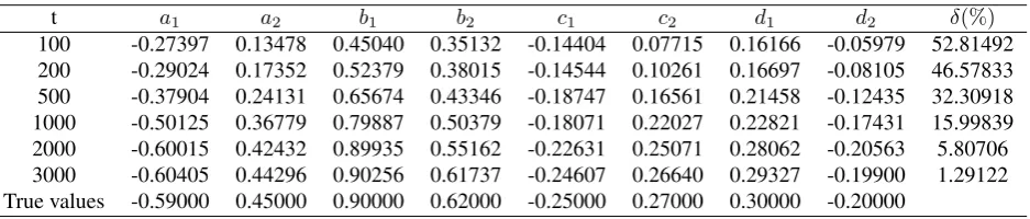
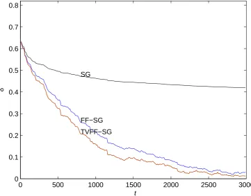
Numerical results are displayed in tables 1, 2, 3 and figure 1. The parameter estimates and their errors with different in-novation length are shown in tables 1, 2 and 3, and the param-eter estimation errorsδ=kθˆ(t)−θk/kθkvs.tare shown in figure 1. In addition, figure 2 shows the time evolution curves of the system parameters vs.tof the TVFF-SG method.

The experiments has been conducted to demonstrate the properties of the proposed algorithm. Some attractive points can be summarized as follows:

(1) The parameter estimation errors of the three algorithms become smaller and smaller astincreasing.

(2) SG doesn’t consider the forgetting factor so that it gets the poorest results.

(3) FF-SG and TVFF-SG both use the forgetting factors to speed up the convergence so they achieve better results than SG.

(4) TVFF-SG estimates have higher accuracy than the other two techniques, etc. SG and FF-SG. This is because that it considers both the tracking ability and the stability of the al-gorithm. This also confirms that the proposed TVFF-SG is effective for parameter identification.

5 Conclusions

This paper investigates the parameter identification of the nonlinear system using a novel time-varying forgetting fac-tor stochastic gradient(TVFF-SG) algorithm. The proposed TVFF-SG method considers both the tracking ability and the stability of the algorithm and takes a proper tradeoff between them. The proposed method is simple and easily to imple-ment in system identification problems. The simulation re-sults verify the effectiveness of the proposed approach. The presented method can also be used to solve other system iden-tification problems.

In order to improve the performance of the algorithm, we can combine it with other system identification methods. For example, we can extend the proposed algorithm to multi-innovation based identification method[27] to improve the parameter estimation accuracy. The proposed method can also combine the filtering technology to identify the parame-ters of the other nonlinear systems.

Acknowledgements

(4)

par-Table 1.The SG estimates and errors.

t a1 a2 b1 b2 c1 c2 d1 d2 δ(%)

[image:4.595.53.530.157.257.2]

100 -0.25643 0.10755 0.41384 0.33316 -0.14659 0.07092 0.16205 -0.05569 56.30533 200 -0.26419 0.12450 0.44625 0.34670 -0.14576 0.08137 0.16283 -0.06424 53.54414 500 -0.28536 0.14612 0.48627 0.36103 -0.15559 0.09841 0.17536 -0.07677 49.49292 1000 -0.30569 0.17490 0.51704 0.36992 -0.14771 0.10897 0.17071 -0.08672 46.33699 2000 -0.32708 0.19692 0.54514 0.37819 -0.14720 0.11824 0.17278 -0.09485 43.38542 3000 -0.33788 0.20963 0.56047 0.38500 -0.14934 0.11979 0.17418 -0.09434 41.81658 True values -0.59000 0.45000 0.90000 0.62000 -0.25000 0.27000 0.30000 -0.20000

Table 2.The FF-SG estimates and errors.

t a1 a2 b1 b2 c1 c2 d1 d2 δ(%)

100 -0.26954 0.12798 0.44137 0.34673 -0.14464 0.07554 0.16169 -0.05871 53.68516 200 -0.28349 0.16094 0.50401 0.37156 -0.14528 0.09701 0.16561 -0.07652 48.36300 500 -0.35597 0.21982 0.61865 0.41566 -0.17942 0.14936 0.20513 -0.11309 36.28997 1000 -0.46405 0.33428 0.74986 0.47299 -0.16999 0.19877 0.21277 -0.15816 21.65130 2000 -0.57771 0.41033 0.87268 0.52780 -0.21269 0.23785 0.26543 -0.19347 8.53179 3000 -0.60217 0.43336 0.90331 0.59785 -0.25448 0.25998 0.29719 -0.18394 2.55572 True values -0.59000 0.45000 0.90000 0.62000 -0.25000 0.27000 0.30000 -0.20000

Table 3.The TVFF-SG estimates and errors.

t a1 a2 b1 b2 c1 c2 d1 d2 δ(%)

[image:4.595.57.528.388.486.2] [image:4.595.59.528.616.716.2]

(5)

0 500 1000 1500 2000 2500 3000 0

0.1 0.2 0.3 0.4 0.5 0.6 0.7 0.8

t

δ

SG

FF−SG

[image:5.595.120.482.110.393.2]

TVFF−SG

Figure 1.The parameter estimation errorsδvs.t.

0 500 1000 1500 2000 2500 3000

−0.8 −0.6 −0.4 −0.2 0 0.2 0.4 0.6 0.8 1

a 1 a₂ b

1

b 2

c 1 c

2 d₁

d₂

t

[image:5.595.112.480.430.740.2]

parameter estimates

(6)

tially supported by the National Natural Science Founda-tion of China(Grant No.11771376) and the Natural Science Foundation of the Jiangsu Higher Education Institutions of China(Grant No.13KJD520010).

REFERENCES

[1] J.P. Norton. An Introduction to Identification, Academic Press, London and New York, 1986.

[2] T. Soderstrom, P. Stoica. System identification, Prentice-Hall, Inc., Englewood Cliffs, NJ, 1989.

[3] L. Ljung. System Identification. Theory for the User, second ed., Prentice-Hall, Inc., Englewood Cliffs, NJ, 1999.

[4] R.V. Herpen, O. Bosgra, T. Oomen. Bi-Orthonormal Polyno-mial Basis Function Framework With Applications in Sys-tem Identification, IEEE Transactions on Automatic Con-trol,vol.61, no.11, 3285-3300, 2012.

[5] G. Pillonetto, T. Chen, A. Chiuso, G.D. Nicolao, L. Ljung. Regularized linear system identification using atomic, nuclear and kernel-based norms, Automatica, vol.69, no.3, 137-149, 2016.

[6] M. Eklund, J. Michael, J. Mclellan. Nonlinear system identi-fication and control of chemical processes using fast orthogo-nal search, Jourorthogo-nal of Process Control, vol.17, no.9, 742-754, 2007.

[7] M.S. Escobar, H. Kaneko, K. Funatsu. Combined gener-ative topographic mapping and graph theory unsupervised approach for nonlinear fault identification. Aiche Journal, vol.61, no.5, 1559-1571, 2015.

[8] M. Mansouri, O. Avci, H. Nounou, M. Nounou. Parameter identification for nonlinear biological phenomena modeled by S-systems International Multi-conference on Systems, 1-6, 2015.

[9] J. Zhang, H. Xu. Online Identification of Power System Equivalent Inertia Constant. IEEE Transactions on Industrial Electronics, vol.99, no.4, 1-2, 2017.

[10] T. Baldacchino, S.R. Anderson, V. Kadirkamanathan. Compu-tational system identification for Bayesian NARMAX mod-elling. Automatica, vol.49, no.9, 2641-2651, 2013.

[11] F. Ding, G. Liu, X.P. Liu. Partially coupled stochastic gra-dient identification methods for non-uniformly sampled sys-tems, IEEE Trans. Autom. Control, vol.55, no.8, 1976-1981, 2010.

[12] Z. Wang, Q. Jin, X. Liu. Recursive least squares identifica-tion of hybrid BoxCJenkins model structure in open-loop and closed-loop. Journal of the Franklin Institute, vol.352, no.2, 265-278, 2016.

[13] M. Liu, Y. Xiao, R. Ding. Newton iterative identification for a class of output nonlinear systems with moving average noises. Applied Mathematical Modelling, vol.37, no.9, 6584-6591, 2013.

[14] J. Yuan, X. Zhang, X. Zhu, E. Feng, H. Yin. Pathway iden-tification using parallel optimization for a nonlinear hybrid

system in batch culture. Nonlinear Analysis Hybrid Systems, vol.15, no.2, 112-131, 2015.

[15] D.Q. Wang, F. Ding, Extended stochastic gradient identi-fication algorithms for HammersteinCWiener ARMAX sys-tems,Computers and Mathematics with Applications, vol.56, no.12, 3157-3164, 2008.

[16] F. Ding, H.Z. Yang, F. Liu, Performance analysis of stochastic gradient algorithms under weak conditions, Science in China Series FCInformation, vol.51, no.9, 1269-1280, 2008.

[17] S. Cheng, Y. Wei, D. Sheng, Y. Chen, Y. Wang. Identifica-tion for Hammerstein nonlinear ARMAX systems based on multi-innovation fractional order stochastic gradient, Signal Processing, vol.142, no.1, 1-10, 2017.

[18] Z. Shi, Y. Wang, Z. Ji. Bias compensation based partially cou-pled recursive least squares identification algorithm with for-getting factors for MIMO systems: Application to PMSMs. Journal of the Franklin Institute, vol.353, no.13, 3057-3077, 2016.

[19] R. Ghazali. Recursive parameter estimation for discrete-time model of an electro-hydraulic servo system with varying for-getting factor, International Journal of the Physical Sciences, Vol.6, no.30, 6829-6842, 2011.

[20] J. Penm. High-Dimensional ARMA Model Identification and Its Application to Healthcare Picture Smoothing Using a For-getting Factor. Applied Mathematical Sciences, vol.4, no.23, 1129-1139, 2010.

[21] R. Lamare, R. Sampaio-Neto. Low-complexity variable step-size mechanisms for stochastic gradient algorithms in mini-mum variance CDMA receivers, IEEE Transactions on Signal Processing, vol.54, no.6, 2302-2317, 2006.

[22] Y. Cai, R. Lamare, M. Zhao, J. Zhong. Low-complexity variable forgetting factor mechanism for blind adaptive con-strained constant modulus algorithms. IEEE transactions on signal processing, vol.60, no.8, 3988-4002, 2012.

[23] S.C. Douglas, V.J. Mathews. Stochastic gradient adaptive step size algorithms for adaptive filtering. International conference on digital signal processing, 142-147, 1995.

[24] B. Jiang, F.N. Chowdhury. Parameter fault detection and esti-mation of a class of nonlinear systems using observers. Jour-nal of the Franklin Institute, vol.347, no.2, 725-736, 2005.

[25] D. Antonio, D.H. Zanette, D. Lopez. Frequency stabilization in nonlinear micromechanical oscillators. Nature Communi-cations, vol.3, no.3, 806-811, 2012.

[26] P.L. Green, K. Worden, K. Atallah, N.D. Sims. The benefits of duffing-type nonlinearities and electrical optimisation of a randomly excited energy harvester. Journal of Sound and Vi-bration, vol.331, no.20, 4504-4517, 2012.