Constrained Optimal Power Flow using Particle Swarm Optimization

(1)

International Journal of Emerging Technology and Advanced Engineering

Website: www.ijetae.com (ISSN 2250-2459, Volume 2, Issue 2, February 2012)

235

Constrained Optimal Power Flow using Particle Swarm

Optimization

C.Kumar

1

, Dr. Ch. Padmanabha Raju

2

1 _{Associate Professor, Department of EEE, PVP Siddhartha Institute of Technology, Vijayawada, A.P, INDIA.}

2 _{Professor, Department of EEE, PVP Siddhartha Institute of Technology, Vijayawada, A.P, INDIA.}

1

[email protected]

2_{[email protected]}

Abstract— Optimal power flow is an optimizing tool for operation and planning of modern power systems. This paper presents the solution of the optimal power flow (OPF) using particle swarm optimization (PSO). The main goal of this paper is to verify the viability of using PSO problem composed by different objective functions. This OPF problem involves the optimization of various types of objective functions while satisfying a set of operational and physical constraints while keeping the power outputs of generators, bus voltages, shunt capacitors/reactors and transformers tap settings in their limits. The proposed PSO method is demonstrated and compared with Evolutionary Programming (EP) approach on the standard IEEE 14-bus system. The results show that the proposed PSO method is capable of obtaining higher quality solutions efficiently in OPF problem.

Keywords— Optimal power flow, PSO, Constraint handling, EP.

I. INTRODUCTION

The Optimal Power Flow (OPF) is an important criterion in today’s power system operation and control due to scarcity of energy resources, increasing power generation cost and ever growing demand for electric energy. As the size of the power system increases, load may be varying. The generators should share the total demand plus losses among themselves. The sharing should be based on the fuel cost of the total generation with respect to some security constraints.

The main purpose of an OPF is to determine the optimal operating state of a power system and the corresponding settings of control variables for economic operation, while at the same time satisfying various equality and inequality constraints. The power flow equations are the equality constraints and the inequality constraints are the limits on control variables and the operating limits of power system dependent variables. A widely considered objective amongst a number of different operational objectives that an OPF problem may be formulated is the fuel cost minimization. Researchers proposed different mathematical formulations of the OPF problem that can be classified into linear, non-linear or mixed integer linear problem [1-3].

In its most general formulation, the optimal power flow problem is a nonlinear, non-convex, large scale, static optimization problem [4,5].Many mathematical programming techniques such as linear programming, nonlinear programming, quadratic programming, Newton method and interior point methods have been applied to solve the OPF problem successfully.

The interior point methods also have major drawbacks such as improper step size selection may cause the sub-linear problem to have a solution that is infeasible in the original nonlinear domain. In addition, a bad initial, termination, and optimality criterion unable interior point methods to solve nonlinear and quadratic objective functions. However, these classical optimization methods are limited in handling algebraic functions.

In recent years, many heuristic algorithms, such as genetic algorithms [6] and evolutionary programming[7,8], simulated annealing[9], particle swarm optimization [10,11], chaos optimization algorithm [12], tabu search [13] have been proposed for solving the OPF problem, without any restrictions on the shape of the cost curves. A genetic algorithm approach is applied for ac-dc optimal power flow problem in [6].

(2)

International Journal of Emerging Technology and Advanced Engineering

236

In this paper, particle swarm optimization algorithm is developed to effectively solve the optimal power flow problem incorporating a set of constraints. Simulations for PSO-OPF are carried out on IEEE 14-bus test systems with different objective functions.

II. PARTICLE SWARM OPTIMIZATION

Particle swarm optimization (PSO) is a population based stochastic optimization technique inspired by social behavior of bird flocking or fish schooling. PSO shares many similarities with evolutionary computation techniques such as Genetic Algorithms (GA). The system is initialized with a population of random solutions and searches for optima by updating generations. However, unlike GA, PSO has no evolution operators such as crossover and mutation. In PSO, the potential solutions, called particles, fly through the problem space by following the current optimum particles. The detailed information will be given in following sections. Compared to GA, the advantages of PSO are that PSO is easy to implement and there are few parameters to adjust. PSO has been successfully applied in many areas: function optimization, artificial neural network training, fuzzy system control, and other areas where GA cannot be applied.

A. PSO Algorithm

Step 1: Generation of initial condition of each agent. Initial searching points (

s

_i0) and velocities (

v

_i0) of each

agent are usually generated randomly within the allowable range. The current searching point is set to pbest for each agent. The best evaluated value of pbest is set to gbest, and the agent number with the best value is stored.

Step 2: Evaluation of searching point of each agent. The objective function value is calculated for each agent. If the value is better than the current pbest of the agent, the pbest value is replaced by the current value. If the best value of pbest is better than the current gbest, gbest is replaced by the best value and the agent number with the best value is stored.

Step 3: Modification of each searching point. The current searching point of each agent is changed using follow equation.

)

(

*

)

(

*

2 2

1 1 1

k i

k i i k

i k

i

s

gbest

rand

c

s

pbest

rand

c

wv

v













(1)

w



w

_max



((

w

_max



w

_min

)

/(

iter

_max

))

*

iter

(2)

1





k1 i k i k

i

s

v

s

₍₃₎

Step 4: Checking the exit condition. The current iteration number reaches the predetermined maximum iteration number, then exits. Otherwise, the process proceeds to step 2.

III. MATHEMATICAL FORMULATION OF OPTIMAL POWER

FLOW PROBLEM

The OPF problem is to optimize the steady state performance of a power system in terms of an objective function while satisfying several equality and inequality constraints. Mathematically, the OPF problem can be formulated as given

Min

F

(

x

,

u

)

(4)

Subject to

g

(

x

,

u

)



0

(5)

0 )

,

(

x

u



h

(6)

where x is a vector of dependent variables consisting of

slack bus power 1

G

P

, load bus voltages

V

_L, generator

reactive power outputs

Q

_G, and the transmission line

loadings

S

_l, Hence, x can be expressed as given

]

...

,

...

,

...

,

[

1 1

1 L LNL G GNG l lnl

G T

S

Q

V

P

x



(7)

where NL,NG and nl are number of load buses, number of generators and number of transmission line respectively .u is the vector of independent variables consisting of

generator voltages VG, generator real power outputs

P

G

except at the slack bus 1

G

P

, transformer tap settings T, and

shunt VAR compensations

Q

_C. Hence u can be expressed

as given

]

...

,

...

,

...

,

...

[

1 2

1 GNG G GNG 1 NT C CNC

G T

Q

T

P

V

u



(8)

(3)

International Journal of Emerging Technology and Advanced Engineering

237 A. Objectives

The objectives considered for minimization are as follows. Objective Function 1: Fuel cost of generating units

(

f

₁) Objective Function 2: Active power loss (

f

₂) Objective Function3: Weighted multi objective function

(

f

₃) where

1

f

=min







NG

i

i Gi i Gi

i

P

b

P

C

a

1 2

)

(

(9)

2

f

=min(

(

2 cos(

)

1

2 2









NL

i

j i j i j i

ij

V

G



) (10)

f

₃



w

₁

*

f

₁



w

₂

*

f

₂ (11)

Here

w

₁



w

₂



1

B. Constraints

The OPF problem has two categories of constraints:

Equality Constraints: These are the sets of nonlinear power flow equations that govern the power system, i.e,

0 )

cos(

1









 j ij ij i j n

j i Di

Gi

P

V

Y

P





(12)

0 )

sin(

1













 j ij ij i j n

j i Di

Gi

Q

V

Y

Q





(13)

Where

P

_Gi and

Q

_Giare the real

and reactive power outputs injected at bus-

i

respectively,

the load demand at the same bus is represented by

P

_Diand

Di

Q

, and elements of the bus admittance matrix are

represented by

Y

_ij and



_ij.

Inequality Constraints: These are the set of constraints that represent the system operational and security limits like the bounds on the following:

1) generators real and reactive power outputs

P

_Gimin



P

_Gi



P

_Gimax

,

i



1 ,



,

N

_G (14)

Q

_Gimin



Q

_Gi



Q

_Gimax

,

i



1 ,



,

N

_G (15)

2) voltage magnitudes at each bus in the network

(16)

3) transformer tap settings

T

i

T

i

T

i

,

i

1 ,

,

NT

max min







(17) 4) reactive power injections due to capacitor banks

Q

_Cimin



Q

_Ci



Q

_Cimax

,

i



1 ,



,

CS

(18)

5) transmission lines loading

S

_i



S

_imax

,

i



1 ,



,

nl

(19)

6) voltage stability index

Lj

i

Lj

i

,

i

1 ,

,

NL

max







(20)

Handling of Constraints: There are different ways to handle constraints in evolutionary computation optimization algorithms. In this paper, the constraints are incorporated into fitness function by means of penalty function method, which is a penalty factor multiplied with the square of the violated value of variable is added to the objective function and any infeasible solution obtained is rejected.

To handle the inequality constraints of state variables including load bus voltage magnitudes and output variables with real power generation output at slack bus, reactive power generation output, and line loading, the extended objective function can be defined as:

)

(

)

(

)

(

)

(

)

(

1 1

1



 





NL

i i s NL

i i v

N

i Gi q

G p N

i Gi i

S

h

K

V

h

K

Q

h

K

P

h

K

P

F

OF

(21)

Where

K

_p,

K

_q,

K

_v,

K

_s are penalty constants for the

real power generation at slack bus, the reactive power generation of all generator buses or PV buses and slack bus, the voltage magnitude of all load buses or PQ buses, and line or transformer loading, respectively.

)

(

P

G1

h

,

h

(

Q

Gi

)

,

h

(

V

i

)

,

h

(

S

i

)

are the penalty

(4)

International Journal of Emerging Technology and Advanced Engineering

238

the voltage magnitudes of all PQ buses, and line or transformer loading, respectively. NL is the number of PQ buses. The penalty function can be defined as:

2 max

)

(

)

(

x

h





, if

x



x

_max

=

(

x

_min



x

)

2, if

x



x

_min

=

0

, if

x

_min



x



x

_max (22)

Where

h

(

x

)

is the penalty function of variable

x

,

x

max

and

x

min are the upper limit and lower limit of variable

x

, respectively.

IV. OVERALL COMPUTATIONAL PROCEDURE FOR SOLVING

THE PROBLEM

The implementation steps of the proposed PSO based algorithm can be written as follows;

Step 1: Input the system data for load flow analysis

Step 2: Run the power flow

Step3: At the generation Gen =0; set the simulation parameters of PSO parameters and randomly initialize k individuals within respective limits and save them in the archive.

Step 4: For each individual in the archive, run power flow to determine load bus voltages, angles, load bus voltage stability indices, generator reactive power outputs and calculate line power flows.

Step 5: Evaluate the penalty functions

Step6: Evaluate the objective function values and the corresponding fitness values for each individual.

Step 7: Find the generation local best xlocal and global best xglobal and store them.

Step 8: Increase the generation counter Gen = Gen+1.

Step 9: Apply the PSO operators to generate new k individuals

Step 10: For each new individual in the archive, run power flow to determine load bus voltages, angles, load bus voltage stability indices, generator reactive power outputs and calculate line power flows.

Step 11: Evaluate the penalty functions

Step12: Evaluate the objective function values and the corresponding fitness values for each new individual.

Step 13: Apply the selection operator of PSO and update the individuals.

Step 14: Update the generation local best xlocal and global best xglobal and store them.

Step 15: If one of stopping criterion have not been met, repeat steps 4-15. Else go to step 16

Step 16: Print the results

There are two stopping criterion for the optimization algorithm. The algorithm can be stopped if the maximum number of generations is reached (Gen = Genmax) or there is no solution improvement over a specified number of generations. The first criterion is used in this paper.

V. SIMULATION RESULTS

The proposed EP and PSO algorithms for solving optimal power flow problems is tested on standard IEEE 14-bus test system. The proposed algorithms are implemented using MATLAB 7.1 running on Pentium IV, 2.66GHz and 512MB RAM personal computer. The EP and PSO parameters used for the simulation are summarized in Table I

TABLEI

OPTIMAL PARAMETER SETTINGS FOR EP AND PSO

Parameter EP PSO

Population size Number of iterations Cognitive constant, c1

Social constant, c2 Inertia weight, W

20 250

- - -

20 150

2 2 0.3-0.95

A. IEEE 14-bus system results

(5)

International Journal of Emerging Technology and Advanced Engineering

239

Evolutionary programming (EP) method has been applied on the IEEE-14 bus system. Here we have considered three objective functions. Objective function-1 is the cost objective function. Objective function-2 is the loss objective function. Objective function-3 is the multi objective function i.e. both cost and losses are taken as objectives. The fitness function is taken as the reciprocal of the objective function.

The proposed PSO algorithm was applied to find the optimal scheduling of the power system for the base case loading condition to minimize specified objective functions. Generator active-power outputs, generator terminal voltages, transformer tap settings and shunt reactive power compensating elements were taken as control variables. The control variables are represented as floating point numbers in the population. The upper and lower voltage limits of load buses were taken as 1.06 and 0.95 respectively.

Table II presents the optimal settings of the control-variables with the three objective functions. From the Table 2, it was found that all the state variables satisfy their lower and upper limits.

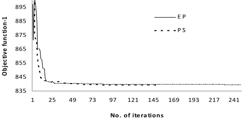
From the Table II, it can be observed that the PSO algorithm is able to reduce the cost of generation less than that of the cost of generation obtained by the EP method. It is also evident from the results that particle swarm optimization technique outperforms in achieving minimum of the specified objective under different network contingencies when compared with evolutionary programming method. Figures 1-4 shows the convergence characteristics of the three objective functions with EP and PSO OPF algorithms. It can be observed that the PSO converges to a minimum value than EP in minimum number of iterations.

835 845 855 865 875 885 895

1 25 49 73 97 121 145 169 193 217 241

No. of ite ra tions

O

b

je

ct

iv

e

fu

n

ct

io

n

-1 E P

P S O

Figure 1 :Convergence of objective function-1

0.015 0.017 0.019 0.021 0.023 0.025

1 26 51 76 101 126 151 176 201 226

No. of itera tions

O

b

je

c

ti

v

e

f

u

n

c

ti

o

n

-2

E P

P S O

Figure 2: Convergence of objective function-2

835 855 875 895 915 935 955 975 995

1 26 51 76 101 126 151 176 201 226

No. of itera tions

O

b

je

c

ti

v

e

f

u

n

c

ti

o

n

-3

(c

o

s

t) E P

P S O

Figure 3: Convergence of objective function-3 (Cost)

0.0485 0.0505 0.0525 0.0545 0.0565 0.0585

1 26 51 76 101 126 151 176 201 226

No.of iterations

O

b

je

c

ti

v

e

f

u

n

c

ti

o

n

-3

(L

o

s

)

E P P S O

[image:5.612.53.299.560.683.2]

(6)

International Journal of Emerging Technology and Advanced Engineering

240 TABLEIII

OPTIMAL SETTINGS OF CONTROL VARIABLES

Control variables

Objective function-1 Objective function-2 Objective function-3

EP PSO EP PSO EP PSO

PG1 PG2 PG3 PG4 PG5

1.1242 0.7000 0.2783 0.2605 0.2778

1.1279 0.7000 0.2749 0.2613 0.2746

0.6138 0.3889 0.8000 0.5019 0.3049

0.2485 0.7000 0.8000 0.5424 0.3163

1.1191 0.7000 0.2728 0.2746 0.2734

1.1278 0.7000 0.2748 0.2627 0.2739 QG1

QG2 QG3 QG4 QG5

0.0100 0.1108 0.1760 0.1283 0.0995

-0.0929 0.0534 0.0373 0.0924 0.1459

0.1796 -0.1906 -0.0342 0.1807 0.0628

0.0741 0.0506 0.1786 0.0044 0.0505

-0.0789 0.1838 0.1688 0.0322 0.1177

-0.0936 0.0574 0.0370 0.1177 0.1782

V1 V2 V3 V4 V5

1.0700 1.0567 1.0275 1.0137 1.0480

1.0700 1.0621 1.0389 1.0598 1.0688

1.0700 1.0541 1.0425 1.0309 1.0387

1.0700 1.0644 1.0541 1.0491 1.0326

1.0700 1.0609 1.0321 1.0564 1.0571

1.0715 1.0621 1.0387 1.0520 1.0784 T1

T2 T3

0.9543 1.0879 1.0157

1.0322 0.9000 0.9922

1.0064 0.9360 1.0473

1.0260 0.9665 0.9669

1.0331 0.9017 0.9617

1.0118 0.9201 1.0004 Qsh1

Qsh2 Qsh3 Qsh4 Qsh5

0.0521 0.0975 0.0191

0 0.0306

0.0260 0.0500 0.0351 0.0500 0.0500

0.0183 0.0098 0.0348 0.0178 0.0399

0.0016 0.0105 0.0389 0.0824 0.0787

0.0369 0.1000 0.0658 0.0364 0.0551

0.0500 0.0500 0.0218 0.0208

0

Cost ($/hr) 840.1141 839.0662 1072.1 1105.4 839.7088 839.2721

Loss (p.u.M.W)

0.0509 0.0488 0.0194 0.0171 0.0499 0.0493

CPU Time (sec)

63.0150 35.5470 60.9060 39.7190 62.9690 41.4690

VI. CONCLUSIONS

In this paper, the application of PSO method for solving optimal power flow problems has been presented. The generation cost and real power losses were reduced through adjustment of generator outputs, generator voltages, tap changing transformers, and shunt compensation. The simulation results on 14-bus system have been presented for illustration purpose. The algorithms EP and PSO were accurately and reliably converged to the global optimum solution in each case. Moreover, the PSO-algorithm is capable of producing better results compared with other algorithms.

REFERENCES

[1] E.Ewald,D.W.Angland, Regional integration of electric power systems,IEEE Spectrom, April 1964 ,pp.96-101. [2] D.Watts, Security & vulnerability in electric power

system,NAPS 2003, 35th North American Power Symposium, University of Missouri-Rolla in Rolla, Missouri, October 20-21, 2003. pp. 559-566.

[3] Bullock, G.C., “Cascading Voltage Collapse in Tennese, August 22, 1987”, Proceedings of 17th Annual

Western Protective Relay Conference", Spokane,

Washington, October 1990.

[4] IEEE Special Publication 90TH0358-2PWR, “Voltage Stability of Power Systems: Concepts, Analytical Tools and Industry Experience", The IEEE Working Group on

(7)

International Journal of Emerging Technology and Advanced Engineering

241

[5] North American Electric Reliability Council, “Survey of the voltage collapse phenomenon”, August 1991. [6] Venikov, V.A., V.A Stroev, V.I. Idelchick, and V.I.

Tarasov, “Estimation of electric power system steady state stability in load flow calculations", IEEE Trans. on PAS, Vol.PAS-94, No.3, May/June 1975, pp.1034-1040.

[7] Lof, P.A., David J. Hill, Stefan Arnborg, and Goran Andersson, "On the Analysis of Long-term Voltage Stability", Electric Power & Energy Systems, Vol.15, No.4, 1993, pp.229-237.

[8] Illiceto, F., E. Cineiri, and L. Casely-Hayford, “Long lightly loaded HV transmission lines to expand electrification of developing countries, application in Ghana", CIGRE, International Conference on Large High Voltage Electric Systems, 29th August-6th September, 1984.

[9] C.A. Canizares, and F.L. Alvarado, “Point of collapse and continuation methods for large AC-DC systems”, IEEE Transactions on power systems, Vol.7, No.1, February 1993, pp.1-8.

[10] H.D. Chiang, A. Flueck, K.S. Shah, N. Balu, “CPFLOW: A practical tool for tracing power system steady-state stationary behavior due to load and generation variations”, IEEE Trans. Power Systems, vol. 10, no. 2, May 1995, pp. 623-634.

[11] S. Greene, I. Dobson, F.L. Alvarado, “Sensitivity of the loading margin to voltage collapse with respect to arbitrary parameters”, IEEE Trans. on power systems, Vol. 12, No. 1, February 1997, pp. 262-272.

[12] C. L. DeMarco, G. C. Verghese, “Bringing phasor dynamics into the power system load flow”, Proceedings 1993 North American Power Symposium, Washington D.C., Oct. 11-12, 1993, pp. 463-471. [13] P Kessel and H Glavitsch, “Estimating the voltage

stability of a power system”, IEEE Trans. on PD, Vol.1, No.3, pp.346-354, 1986 [49]

[14] Kennedy I. and Eberhart R. C., “Particle swarm optimization,” Proceedings of IEEE International Conference on Neural Networks, Piscataway, NJ. pp. 1942-1948, 1995.