2017 2nd International Conference on Computer, Mechatronics and Electronic Engineering (CMEE 2017) ISBN: 978-1-60595-532-2
Continuous Approximation of Nonlinear L
1Problem
Based on BP Neural Network
Bing-jiang ZHANG
School of Applied Science, Beijing Information Science and Technology University, Beijing, China
Keywords: Nonlinear L1 Problem, Analyticity, Neural network.
Abstract. The nonlinear L1 problem is a non-differentiable optimization problem. The objective function of nonlinear L1 problem is continuously approximated by using the characteristics of neural network in order to make it continuously differentiable. A concrete algorithm for approximation of continuous functions at the discontinuity of the objective function is given based on the principles of BP neural network, and then the effectiveness of the method is verified by a specific example.
Introduction
The mathematical model of nonlinear L1 problem is usually expressed as
(P1)
( )
R
=1
min ( ) | |
n
m
i x
i
F x f x
∈
=
∑
, (1)where
(
)
n1, 2, , n R
x= x x x ∈ ,
( )
( 1, 2, , ) if x i= m are defined as continuously differentiable functions on
Rn and at least one function in it is nonlinear [1]. It is obvious that there is no continuity in the change of the objective function in (P1).
Some effective algorithms for such a problem have been given by domestic and foreign scholars since 1987 based on the entropy function method [2-4] and good results have been achieved. The development of computer technology in recent years has also contributed to rapid development of some swarm intelligence algorithms. In [5], Particle Swarm Optimization is used to solve the problem of nonlinear modular minimization and better numerical results are obtained. In [6], a new smoothing approximation function for nonlinear L1 problem is given, which has a simple form and good numerical stability. This paper attempts to establish a model using neural network to continuously approximate the objective function of the L1 problem to endow it with good analyticity.
The data before and after the point of discontinuity is a discrete ordinal data for the objective functions fi
( )
x (i=1, 2,,m). Assuming the first s sample sets of discrete data are h, o=g h( )
, where(
)
T1, 2, ,
h= h− h− h−i , g is a nonlinear continuous function, i.e. the function obtained by continuous
approximation at the point of discontinuity. The required continuous function can be obtained as long as the right function g is confirmed. However, it is very difficult to characterize the continuous changes of this nonlinear function due to its complexity. And the continuous function approximation itself is a multi-input and single-output nonlinear mapping. This paper chooses BP neural network modeling and continuously approximates the objective function for such a nonlinear relationship.
In this paper, BP neural network modeling is used, the input sample set is
(
)
T 1, 2, ,h= h− h− h i− ,
the output set is o, and some matching pairs are selected as the training samples, such as
(
h l,)
. The function g after learning is the desired nonlinear continuous function.Learning Process of BP Neural Network
BP neural network trains and establishes the network through the error back propagation algorithm with the known learning samples. Its learning process is divided into forward propagation and back propagation.
Step 1 Set the initial connection weights of the nodes between adjacent layers of the network and set the initial thresholds of the nodes between the hidden layer and the output layer. The random small value between (-1, 1) is usually selected for the initial weights and thresholds.
Step 2 Select and input training samples.
Step 3 Confirm the activation function of the input information in the forward propagation process, where the S activation function [4] is used, namely
( )
11 x
f x
e−
=
+ . (2)
The output vector y kk( =1, 2,…,H) is obtained at the output layer’s node after the activation of the S activation function.
1
L
k jk j k j
y f µ y ψ
=
′
= −
∑
, (3) where1
M
j ij i j i
y f W x θ
=
′ = −
∑
. (4)j
y′ is the output vector obtained in the hidden layer’s node j j( =1, 2,…, )L ;
k
ψ and θj respectively represent the threshold of the output node K and the hidden layer’s node j; µjkrepresents the connection weight between the hidden layer’s node j and the output layer’s node k; Wij represents the connection weight between input node i i( =1, 2,…,M)
and the hidden layer’s node j; xi is the feature vector at the input layer’s node i.
Step 4 Calculate the error between the training output yk and the target output Tk:
(
) (
1)
k yk Tk yk yk
δ = − − . (5) Step 5 Return the error δk along the original channel for back propagation and then calculate the hidden layer error:
(
)
1
1 H
k k jk j k
y y
γ δ µ
=
′ ′
= −
∑
. (6) Step 6 Adjust the weight µjk and the threshold ψk along the direction of error reduction:jk jk c kyj
µ =µ + δ′ ′, (7)
k k d k
ψ =ψ + δ . (8) Step 7 Adjust the weight Wij and the threshold θj along the direction of error reduction:
ij ij j i
W =W +c xγ , (9)
j j d j
θ =ψ + ⋅γ . (10) Step 8 learn the above process repeatedly for each sample in the training sample set, and stop the operation until the mean square error of the whole sample set
(
)
2 11 M
lk k t
E y T
N =
=
∑
− . (11)In Equation (2.10) ylk is the output value obtained during the learning process.
Approximation Algorithm of Continuous Function Based on Neural Network
The BP neural network has the effect of function approximation as it has been proved theoretically to have the ability to process complex nonlinear signals. For any nonlinear function : Rn Rm
g →
there is a BP neural network which can approximate to g by an arbitrary accuracy. In other words, with any given set of training samples, assuming the set of input signals is X and the set of output signals is Y, and then there is a mapping relationship between them : Rn Rm
g → , making Y =g X
( )
. The mapping will be nonlinear if the neural network is considered to be a mapping from input to output. If the number of the input nodes is n and that of output nodes is m, then the network is a mapping from Rn to Rm, which is: Rn Rm
G → , Y=G X
( )
. The key lies in how to design a neural network so that themapping G can be the best approximation of the mapping g. The method of neural network avoids the difficulty in choosing the function and solving coefficients. It can realize the approximation of complex continuous functions only by fitting the nonlinear function.
The concrete algorithm of BP neural network used in the continuous function approximation is as follows:
Step 1 Set initial weights, thresholds and error functions E and confirm the number of input nodes
n, number of output nodes m, number of layers of the neural network, number of hidden layers and number of nodes in each hidden layer.
Step 2 Analyze the point of discontinuity of the objective function in (P1) and extract the training samples; segment the sample data which usually includes learning samples and test samples.
Step 3 Confirm the transfer function and the training function. We need to pay attention to the following two points:
1. The output function should be high order derivative one due to the back propagation of weights. The rate of convergence of the whole model should also be considered. Therefore, the sigmoid function is generally selected for the hidden layer’s output function. Furthermore, the output of the whole network can be any arbitrary value if the final layer uses the purelin function as the activation function since the BP network characteristics of the last layer of neuron can confirm the output characteristics of the neural network as a whole. So, the S function is selected for the hidden layer’s transfer function and linear function for the output layer’s transfer function.
2. There are many training functions of BP neural network in software Matlab. In general, trainlm is used as training function defaulted in the software system.
Step 4 Calculate the expected output according to formulas (2) and (4) and calculate the error between the expected output and the actual output according to formulas (5) and (6). Stop the calculation if the error meets the requirements. If not, start from Step 5.
Step 5 Adjust the weights and thresholds of the output layer and hidden layer according to the error obtained by calculation according to formulas (7) and (10).
Step 6 Stop the calculation if the specified learning times are reached. If not, repeat from Step 3. Step 7 Test the trained network with the test data. Approximate the nonlinear continuous function with the trained network if the testing effect is very good. Otherwise, adjust the structure of the network and repeat the last step until a better test result is obtained.
Numerical Examples
For nonlinear L1 problems
( )
3
i=1
min ( ) | i | x R∈ F x =
∑
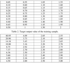
f x ,Analyze the point of discontinuity of the problem and the point of discontinuity of the nonlinear problem is x= ±1. The algorithm is illustrated with only one point as an example below. The training samples are intercepted at the point x=1 and the results are shown in Table 1 and Table 2.
Table 1. Input value p of the training sample.
0.05 0.55 1.05 1.55 0.10 0.60 1.10 1.60 0.15 0.65 1.15 1.65 0.20 0.70 1.20 1.70 0.25 0.75 1.25 1.75 0.30 0.80 1.30 1.80 0.35 0.85 1.35 1.85 0.40 0.90 1.40 1.90 0.45 0.95 1.45 1.95
[image:4.612.162.450.130.389.2]0.50 1 1.50 2
Table 2.Target output valueof the training sample.
40.95 4.09 2.05 2.55 20.90 3.73 2.10 2.60 14.18 3.43 2.15 2.65 10.80 3.16 2.20 2.70 8.75 2.92 2.25 2.75 7.37 2.70 2.30 2.80 6.36 2.50 2.35 2.85 5.60 2.32 2.40 2.90 4.99 2.16 2.45 2.95 4.50 2.00 2.50 3.00
[image:4.612.93.519.518.717.2]Herein, the number of hidden layer’s neurons in the network is 12 and S tangent function is selected for the hidden layer’s output function and the purelin function is selected for the output function of the output layer’s neuron. The trainlm is applied as the training function. The maximum number of trainings is 100 and the global minimum error is 0.005. The global error can reach 0.00498 during the sixty-seventh training according to calculation, which meets the minimum error requirement. The calculation results are shown in Table 3. The approximation process of nonlinear continuous function is shown in Figure 1. The comparison between the simulation value and the target value which is the fitting of the nonlinear continuous function is shown in Figure 2.
Table 3.Calculation results.
Weights of the input
layer to the middle layer (3.36,3.36,-3.36,-3.36,3.36,3.36,-3.36,-3.25,2.21,0.93,2.89,-13.96,2.39) Thresholds of each
neuron in the middle
layer (-33.60,-30.55,27.49,-24.44,-21.38,18.33,15.33,-12.81,-10.35,-0.12,-0.11,10.34) Threshold of each
neuron in the output layer
9.66
Figure 2. Fitting of the continuous function.
Conclusions
In this paper, the objective function of nonlinear L1 problem is continuously approximated by BP neural network so that the obtained approximation function has better analyticity in solving nonlinear problem L1. It can be seen through analysis and verification of practical examples that the BP neural network is effective for the continuity of nonlinear L1 problem.
In addition, BP neural network itself has some defects even if it has been widely applied. Firstly, the rate of convergence of the network is slow due to the fixed learning rate. As a result, it takes long training time. The training time required by the BP algorithm may be very long, as the learning rate scale needs to be improved. Varying learning rate or adaptive learning rate can be adopted. Moreover, the value obtained by BP algorithm cannot always be the global minimum. It may be a local minimum. The additional momentum method can be used to solve the problem.
Acknowledgement
The research was supported by the National Natural Science Foundation of China (Grant No. 60972115) and Beijing Excellent Talent Training Project (Grant No. 2013D005007000003).
Reference
[1] Chris Charalambous, on conditions for optimality of the nonlinear L1 problem, Math Programming. 17 (1997) 123-135.
[2] Qiao C, Yoo M, Optical burst switching-a new parading for an optical internet, Journal of High Speed Networks, Speclai Issue on Optical Networks. 8 (1999) 69-84.
[3] Turner S J, Terabit burst switching, High Speed Networks. 8 (1999) 3-16.
[4] Xiong Y, Vandenhoute M, Cankaya H C, Control architecture in optical burst switching WDM networks, IEEE JSAC. 18(2000) 1838-1851.
[5] Tan S K, Mohan G, Chua K C, Burst rescheduling with wave length and last-hop FDL reassignment in WDM optical burst switching networks, ICC, IEEE, International Conference, 2 (2003).
[6] Wang Ruopeng, Xu Hongmin, Smooth approximation method for nonlinear L1 problem, Pure and Applied Mathematics. 29(2013) 25-32.
[8] Chen Jin-sai, Zhang Xin-bo, Short-term Power System Load Forecasting Based on Improved BP Artificial Neural Network, Journal of Hangzhou Dianzi University. 31(2011) 173-176.