Munich Personal RePEc Archive
Size Distributions for All Cities: Which
One is Best?
González-Val, Rafael and Ramos, Arturo and Sanz,
Fernando and Vera-Cabello, María
13 March 2013
Online at
https://mpra.ub.uni-muenchen.de/45019/
Size Distributions for All Cities: Which One is Best?
Rafael González-Vala
Arturo Ramosb
Fernando Sanzb
María Vera-Cabellob
a
Universidad de Zaragoza & Institut d’Economia de Barcelona
b
Universidad de Zaragoza
Abstract
This paper analyses in detail the features offered by three distributions used in urban
economics to describe city size distributions: lognormal, q-exponential and double
Pareto lognormal, and another one of use in other areas of economics: the log-logistic.
We use a large database which covers all cities with no size restriction in the US, Spain
and Italy from 1900 until 2010, and, in addition, the last available year for the rest of the
countries of the OECD. We estimate the previous four density functions by maximum
likelihood. To check the goodness of the fit in all periods and for the thirty-four
countries we use the Kolmogorov-Smirnov and Cramér-von Mises tests, and compute
the Akaike Information Criterion (AIC) and the Bayesian Information Criterion (BIC).
The results show that the distribution which best fits the data in most of the cases
(86.76%) is the double Pareto lognormal.
Keywords: city size distribution, double Pareto lognormal, log-logistic, q-exponential, lognormal
1
1. Introduction
The study of city size distribution has a long tradition in urban economics. To cite just a
few examples, see Rosen and Resnick (1980), Black and Henderson (2003), Ioannides
and Overman (2003), Soo (2005), Anderson and Ge (2005), and Bosker et al. (2008).
These distributions have an interest beyond the purely statistical, essentially for two
reasons, which feed back to and influence each other. First, because city size
distribution defines the resulting economic landscape. It may be more concentrated or
dispersed, or biased towards an excessive number of large or small centres, with cities
which are similar or very different in size, and all of this has a direct impact on the
spatial distribution of income, on public investment in infrastructure of various kinds in
certain areas, and on imbalances between territories in general. And second, because
this size distribution is susceptible to change over time, according to certain, essentially
economic, incentives.
Over the years, the Pareto distribution (Pareto, 1896) has generated a huge amount of
research and greater acceptance. Considering the rank r (1 for the most populous city, 2
for the second, and so on) of the N cities, we can obtain the expression for the Pareto
distribution usually estimated,
ln
r
=
const
.
−
b
ln
x
, (1)which relates the logarithm of rank with the logarithm of the size of the cities if they
follow a Pareto distribution. In the case of b=1, we obtain the well-known Zipf’s law
(Zipf, 1949) or rank-size rule (see the surveys on this subject by Cheshire, 1999, and
Gabaix and Ioannides, 2004).1
1
2 In an important paper regarding city size distributions, Eeckhout (2004)
essentially proposes three ideas: (1) that when all cities are taken, without any size
restriction, Pareto’s distribution breaks down and the best representation of the data is a
lognormal function; (2) as a theoretical result, if the underlying distribution is
lognormal, which generates a concave rank-size plot, the Pareto exponent decreases
with sample size, meaning that a sample size can be found which verifies Zipf’s law
exactly (these first two contributions clearly show the importance of taking all cities, as
to do otherwise can lead to biased or spurious results); and (3) the data for all US cities
in 1990 and 2000 support the hypothesis of lognormality and the fulfilment of Gibrat’s
law, or the law of proportionate growth, something which was already anticipated from
a theoretical viewpoint by Gibrat (1931) and Kalecki (1945). As a consequence, there
has been a revival of interest in the lognormal distribution, proposed a long time ago as
a good description of city size distribution (Parr and Suzuki, 1973).
Moreover, other statistical distributions have been proposed in studying city
size: the q-exponential distribution (Malacarne et al., 2001; Soo, 2007) and double
Pareto lognormal distribution (Reed, 2002, Giesen et al., 2010). Ioannides and Skouras
(2013) have even proposed a new distribution function which switches between a
lognormal and a power distribution. There is also an older literature that explores
alternative functional forms; see, for example, Cameron (1990), Hsing (1990) or
Kamecke (1990). This paper is in line with all this literature.
With respect to the q-exponential distribution, Malacarne et al. (2001) show
that, when all cities are taken, it has a very close fit to the data. They use data from
American and Brazilian cities. As far as we know, the only other work to test this
statement is that of Soo (2007) who, taking the largest cities of Malaysia (over 10,000
3 us to think, as with the lognormal, that this distribution is suitable when no truncation
point is defined.
The double Pareto lognormal distribution proposed by Reed (2001) has strong
theoretical foundations. Reed (2002) fits the distribution to the smallest settlements of
two US states (West Virginia and California) in 1998 and two Spanish provinces
(Cantabria and Barcelona) in 1996, obtaining good results. The recent paper by Giesen
et al. (2010) shows that the double Pareto lognormal almost always offers a better
description than the lognormal of the city size data for eight countries (Brazil, the Czech
Republic, France, Germany, Hungary, Italy, Switzerland, and the US) in the first decade
of the 21st century, offering the strongest evidence in favour of the double Pareto
lognormal to date.
Apart from these three distributions (the lognormal, the q-exponential and the
double Pareto lognormal), we have observed that the log-logistic distribution also offers
a close description of the data. Thus we add it to the study. The log-logistic has been
used as a simple model of the distribution of wealth or income by Fisk (1961); hence
the name of Fisk distribution in economics. In other fields, it is widely used in survival
analysis when the failure rate function presents a unimodal shape; it has also been used
in hydrology to model stream flow and precipitation. However, to the best of our
knowledge, this is its first appearance in urban economics.
Recently much more complete databases have been constructed, which enable us
to bring more statistical information to bear on the problem dealt with in this work.
Specifically, González-Val (2010) considers all the cities in the US during the entire
20th century; González-Val et al. (2012) do the same for Spain and Italy, as well as for
the US. If these data are used to represent the logarithm of the rank against the
4 opening the way for the consideration of non-Pareto distributions. What we want to
emphasise is that, except for Eeckhout (2004) and Giesen et al. (2010), no previous
studies have considered the entire distribution of cities2, as all of them impose a
truncation point, either explicitly by taking cities above a minimum population
threshold, or implicitly by working with MSAs3. This is usually due to a practical
reason of data availability. Furthermore, these few studies focus only on static city size
distributions in one or two periods, as data over time is rarely available.
Against this background, the first aim of this article is to estimate the density
functions of the double Pareto lognormal, the lognormal, the q-exponential and the
log-logistic for describing city size distributions. Second, we perform standard statistical
tests to assess when the proposed distributions have a close fit to the empirical ones.
Third, standard AIC and BIC information criteria are computed to discriminate in an
accurate way between the four distributions. In any case, as far as we know, this is the
first time that these matters have been subjected to empirical testing with such
comprehensive databases. On the one hand, we use un-truncated city population data;
on the other hand, we take into account in an explicit way the temporal dimension
(considering data from more than a hundred years for three countries: the US, Spain and
Italy, a time span which can be considered as a long-term study) as well as the
geographic or spatial dimension (we analyze data from the last census of the 34
countries of the OECD, a cross-sectional sample of countries comprising many different
urban systems).
2
Michaels et al. (2012) use data from minor civil divisions (MCDs) to track the evolution of population across both rural and urban areas in the United States from 1880 to 2000.
3
5 The article is organised as follows. The second section recalls the definition and
main properties of the four distributions studied. The third summarises and explains the
databases used. Section four shows the results. In section five we discuss the main
results. Finally, section six concludes.
2. Description of the distributions
2.1. The lognormal distribution (ln)
The probability density function (pdf) of the lognormal is given by:
0
,
2
1
)
(
2 2 2 ) (ln>
=
− −x
e
x
x
f
x σ μπ
σ
, (2)where μ and σ2 are the mean and variance of lnx, which in this case denotes the
natural logarithm of the population of the cities. The expression of the corresponding
cumulative distribution function (cdf) is:
⎟
⎠
⎞
⎜
⎝
⎛
−
+
=
2
ln
2
1
2
1
)
(
σ
μ
x
erf
x
cdf
, (3)where erf denotes the error function associated with the normal distribution.
The lognormal distribution has been considered for many years to study city size
(see Richardson, 1973, and references therein). More recently, Eeckhout (2004)
estimates the lognormal distribution, with no truncation point, to study city size in the
US. He defines an equilibrium theory of local externalities as a process generating data
of such a distribution, and justifies the coexistence of proportionate growth and the
resulting lognormal distribution.
2.2. The q-exponential distribution (qe)
6 1
1
( )
1
,
0
q q
a
q
f x
ax
x
q
q
−
⎛
−
⎞
=
⎜
+
⎟
>
⎝
⎠
, (4)where a>0 and q>1are parameters and x denotes the population of the cities. The
expression of the corresponding cumulative distribution function is:
q
ax
q
q
x
cdf
−
⎟⎟
⎠
⎞
⎜⎜
⎝
⎛
+
−
−
=
11
1
1
1
)
(
. (5)In the case that q→1, f(x)→ae−ax, a property which justifies the name of q
-exponential.
This distribution has been used extensively by Tsallis (1988) and his group of
collaborators, arguing for its theoretical applicability to systems with long-range
interactions (Malacarne et al., 2001, can be included in this line of argument). Soo
(2007) uses this distribution to study city size in the case of Malaysia, obtaining low
descriptive performance probably due to the fact that he uses a cut-off of 10,000
inhabitants to define the cities. However, the q-exponential is a particular case of the
distribution known as generalised type II Pareto, which has been considered in various
earlier works (for example, Hosking and Wallis, 1987; Grimshaw, 1993; Choulakian
and Stephens, 2001).
2.3. The double Pareto lognormal distribution (dPln)
The probability density function of the double Pareto lognormal distribution (see Reed,
7
2 2 2
2 2 2
ln( )
( )
exp
1
2 (
)
2
2
ln( )
exp
1
2 (
)
2
2
x
f x
x
erf
x
x
x
erf
x
α βαβ
αμ
α σ
μ ασ
α β
σ
αβ
βμ
β σ
μ βσ
α β
σ
−
⎛
⎞
⎛
⎞
⎛
− −
⎞
=
⎜
+
⎟
⎜
+
⎜
⎟
⎟
+
⎝
⎠
⎝
⎝
⎠
⎠
⎛
⎞
⎛
⎞
⎛
− +
⎞
−
⎜
−
+
⎟
⎜
⎜
⎟
−
⎟
+
⎝
⎠
⎝
⎝
⎠
⎠
(6)wherex>0 and , , ,α β μ σ >0 are the distribution parameters. The dPln distribution has
the property that it follows different power laws in its two tails, namely f x( )≈x− −α 1
when x→ ∞ and f x( )≈xβ −1 when x→0, hence the name of double Pareto. The
central part of the distribution is approximately lognormal, although it is not possible to
exactly delineate the lognormal body part and the Pareto tails (Giesen et al., 2010).
The expression of the corresponding cumulative distribution function is:
2 2 2
2 2 2
1
ln( )
( )
1
2
2
ln( )
exp
1
2(
)
2
2
ln( )
exp
1
2(
)
2
2
x
cdf x
erf
x
x
erf
x
x
erf
α βμ
σ
β
αμ
α σ
μ ασ
α β
σ
α
βμ
β σ
μ βσ
α β
σ
−
⎛
⎛
−
⎞
⎞
=
⎜
+
⎜
⎟
⎟
⎝
⎠
⎝
⎠
⎛
⎞
⎛
⎞
⎛
− −
⎞
−
⎜
+
⎟
⎜
+
⎜
⎟
⎟
+
⎝
⎠
⎝
⎝
⎠
⎠
⎛
⎞
⎛
⎞
⎛
− +
⎞
−
⎜
−
+
⎟
⎜
⎜
⎟
−
⎟
+
⎝
⎠
⎝
⎝
⎠
⎠
(7)The dPln distribution arises as the steady-state distribution of an evolutionary
process of a simple stochastic model of settlement formation and growth based on
Gibrat’s law and a Yule process; see Reed (2002) for details. For more recent work on
an economic model which incorporates the stochastic derivation of Reed (2002), see
Giesen and Suedekum (2012a). The key in this latest model is the endogenous city
creation and the resulting age heterogeneity in cities within the distribution. Giesen and
Suedekum (2012a) argue that Eeckhout’s (2004) theoretical framework and the
lognormal distribution represent a particular scenario of their model, the case when
8
2.4. The log-logistic distribution (ll)
The probability density function of the log-logistic distribution is:
2
ln( )
exp
( )
,
0
ln( )
1 exp
x
f x
x
x
x
μ
σ
μ
σ
σ
−
⎛
−
⎞
⎜
⎟
⎝
⎠
=
>
⎛
+
⎛
−
−
⎞
⎞
⎜
⎟
⎜
⎝
⎠
⎟
⎝
⎠
(8)where μ σ, >0 are the distribution parameters. This pdf can be written in other
mathematically equivalent ways, but we have chosen this form to compare it with that
of the ln and dPln (see Singh and Maddala, 2008, for references and for derivations of
the log-logistic distribution). The cumulative distribution function can be written as:
1
( )
ln( )
1 exp
cdf x
x
μ
σ
=
−
⎛
⎞
+
⎜
−
⎟
⎝
⎠
. (9)
Although there is no specific theoretical foundation for the log-logistic, Hsu (2012)
develops a model of central place theory using an equilibrium entry model to generate a
Pareto upper tail in the city size distribution if the distribution of scale economies is a
regularly varying function. This class of distributions includes the log-logistic.4 As
shown in the fourth section, the log-logistic provide a better fit to empirical city size
data than the other studied distributions in some cases.
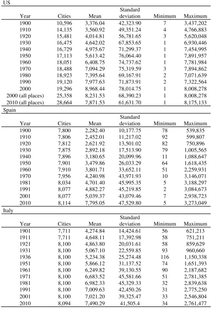
3. The databases
We use un-truncated city population data from all OECD member countries. We
have taken the data corresponding to the last available census for each country, though
for the US, Spain and Italy the data corresponding to the census of each decade of the
20th century is also included. Table 1 shows the number of cities for each decade for
4
9 these last three countries, and the descriptive statistics, and Table 2 reports the number
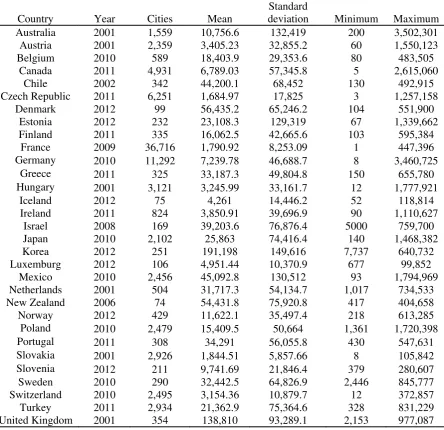
of cities and the descriptive statistics for the remaining OECD countries.
The data on the geographical unit of reference of all countries comes from the
official statistical information services. The urban unit considered is the lowest spatial
subdivision, so they represent the whole territory of the country, with the exception of
Israel, Ireland and the United States; the first because data is only available for
municipalities with more than 5,000 inhabitants; the second because only incorporated
places are taken into account until 20005 (they represent 46.99% of the total population
of the US in 1900 and 61.49% in 2000); and the third because legal towns have
expanded beyond their legally defined boundaries and, as a result, a high number of
persons in the communities is excluded. So, while there are problems of international
comparability, because the administrative definition of a city varies from one country to
another, they do have the major advantage that the size distribution of these ‘legal’
cities comprises, in general, 100% of the population of each country.
This dataset considered is motivated, first, by the availability of a large number
of countries in order to confirm the robustness of our results across countries but,
second, also by the possibility of comparing the time evolution of the urban structure in
three countries; Spain and Italy, as two examples of consolidated and old urban
structures, in contrast to the US, a “young” country whose inhabitants are characterised
by high mobility (Cheshire and Magrini, 2006). Moreover, unlike Italy and Spain,
where urban growth is produced by the increase in population living in existing cities, in
the US urban growth has a double dimension: as well as increases in city size, the
5
10 number of cities almost doubles in the period considered, with potentially different
effects on city size distributions. Therefore, our databases seem to offer an excellent
opportunity to test empirically the Giesen and Suedekum (2012a) and Eeckhout (2004)
models and the influence of city creation on the shape of the city size distribution.
4. Results
4.1. Estimation of the distributions
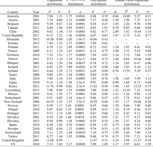
Maximum likelihood (ML) is a standard technique which allows the estimation
of the parameters of distributions given a sample of data. Out of the four distributions
used in this article, only one has a closed form for the corresponding estimators, namely
for the lognormal. The estimators for
μ
andσ
are, respectively, the mean and standarddeviation of the logarithm of the data. For the q-exponential, double Pareto lognormal
and log-logistic we must use numerical methods in order to maximise the log-likelihood
value for each sample. However, the log-likelihood functions to be maximised are easy
to find: see Reed and Jorgensen (2004) for the dPln and Shalizi (2007) for the qe. The
case of ll can be treated in a similar fashion. The results of the estimations are shown for
a selection of years in Table 36.
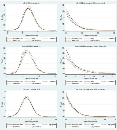
Figure 1 offers a first visual approximation of the goodness of the fit provided
by the four proposed distributions (ln, qe, dPln and ll) to describe empirical city size
distributions. We have taken the last available year of the US, Spain and Italy. We
obtain similar graphs for the rest of the years and different countries.7 Thus, the figure
shows the density kernel estimate of the empirical distribution using an adaptive kernel
compared with the four distributions with the parameters estimated by ML. As in Levy
(2009) and (Giesen et al., 2010), a zoom for the upper tail distribution is also shown.
6
The complete estimation results are available from the authors upon request.
7
11 It is hard to find in Figure 1 any strong differences between the four competing
distributions because all of them capture reasonably well the shape of the empirical one.
Therefore, to be able to discriminate between the four functions, numerical methods and
tests are required rather than graphical tools. Only in this way can we conclude which
one is dominant (although the differences between them are very small) and, thus,
which of the urban theories that are behind the distributions studied (see Sections 1 and
2), are confirmed by the empirical data. This analysis is performed in Subsections 4.2
and 4.3.
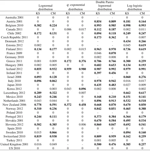
4.2. Standard statistical tests
In this subsection we aim to provide independent tests in order to verify the goodness of
the fit in all cases. We have chosen the Kolmogorov-Smirnov (KS) test, which is
mentioned in a study of similar characteristics to ours (Giesen et al., 2010) and is
standard in the literature, and also the Cramér-von Mises (CM) test. The reason for
including this second test is that its statistic measures the sum of the squared deviations
of the cdf tested with respect to the empirical one. Thus, this statistic has an
interpretation similar to Figures 2a, 2b and 2c in Giesen et al. (2010) and, in this way,
they give similar information. Consequently, here we only show the p-values of the CM
test.8 Moreover, the KS and CM tests have similar power: it is quite low for small
sample sizes but very high for large ones (Razali et al., 2011). Both tests are extremely
precise for large and very large sample sizes, not rejecting the null hypothesis just
because of very small deviations. We recall that the null hypothesis of both KS and CM
tests is that the empirical and the estimated statistical cdfs of the two samples are equal.
8
12 Table 4 reports the cross-sectional evidence. It shows the p-values of both tests
for our sample of the OECD countries, including the first decade of the 21st century for
the US, Spain and Italy. The cases in which the statistical distribution cannot be rejected
at the 5% significance level are highlighted in bold. Looking at the columns of the table
corresponding to each distribution, the qe shows the highest number of rejections (59
out of 66 contrasts performed, 89.39%). The second worst distribution is the ln (60.29%
of rejections), followed by the ll (39.71%); the best distribution is the dPln, which can
only be rejected in 18.51% of the tests performed.
Reading the table by rows, we can observe that there are countries in which the
four distributions can be rejected by both the KS and CM tests (Australia 2001,
Germany 2010, Poland 2010, Spain 2010, Turkey 2011 and the US 2010), while in
others none of the distributions can be rejected by any of the tests (Iceland 2012 and
New Zealand 2006). The former group of six countries have a high number of cities,
while the latter pair are the two countries with the lowest sample size. In general,
although there are some counter-examples, the number of rejections tends to increase
with sample size, something that could be anticipated because the power of the KS and
CM tests increases with sample size.
From a long-term perspective, the results for the US, Spain and Italy during the
twentieth century are summarized as follows. The significance level is always 5%. For
the US and Spain, the four distributions are rejected by both KS and CM in almost all
years; the only exception is the dPln in 1900 and 1920 for the US using the CM test. In
Italy the qe is always rejected, the ln almost always, the ll can never be rejected except
in 1901, 2001 and 2010, and the dPln cannot be rejected in any case except in 1901. The
13 century can be explained by the high sample sizes: since the beginning of the century
these countries have comprised a high number of cities, compared to other countries.
In summary, considering the overall results of the tests for each distribution (the
sum of cases of non-rejections), it follows that the distributions which best fit the data
(out of the four studied here) are, in descending order, the double Pareto lognormal, the
log-logistic, followed closely by the lognormal, and finally the q-exponential.
Therefore, a distribution which has been proposed in the literature, the q-exponential, is
clearly outperformed by others more recently proposed, such as the double Pareto
lognormal and the log-logistic.
4.3. Information criteria
In order to discriminate between the studied distributions, here we take another
approach. We compute two information criteria that are very well suited to the
maximum likelihood method which we have used previously to estimate the parameters
of the four distributions studied: the Akaike Information Criterion (AIC) and Bayesian
Information Criterion (BIC; see, e.g., Giesen et al., 2010, and references therein). The
results are shown in Table 5 for the sample of the OECD countries. Tables 6, 7 and 8
report the results for the US, Spain and Italy, respectively. The interpretation is easy: the
distribution with the lower numerical value out of the AIC or BIC is favoured. In
general, the outcomes confirm most of the results obtained from the statistical tests
carried out in Subsection 4.2.
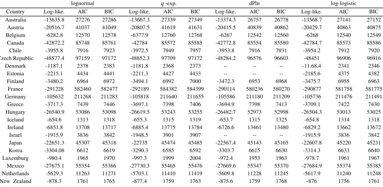
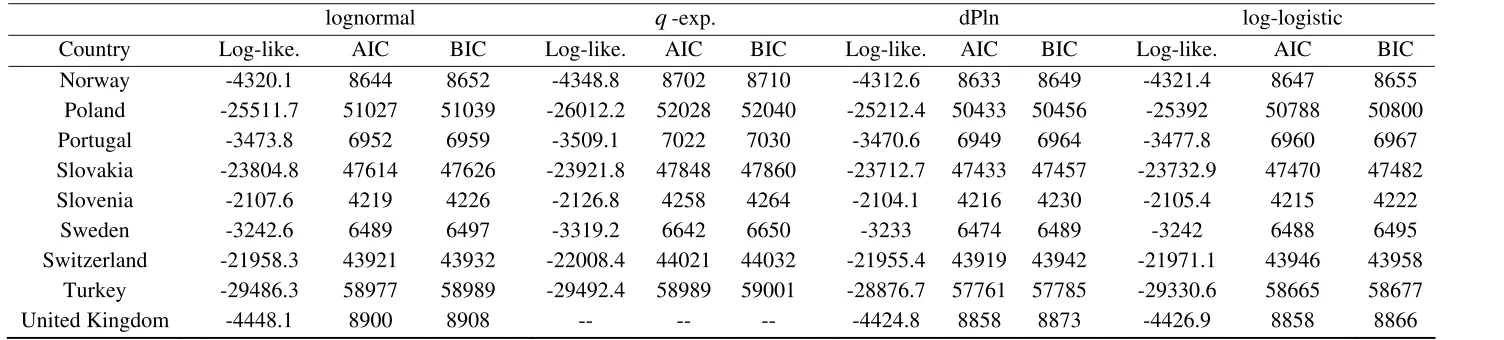
Regarding the cross-sectional evidence (Table 5), in most of the cases (25
countries) there is a coincidence between the AIC and BIC in the selection of the best
fit. The discrepancies appear in Finland (2011), Greece (2011), Mexico (2010), Portugal
14 dPln, while the BIC selects the ln three times, the ll two times and the qe one time. In
these six situations when the criteria do not agree, we follow Burnham and Anderson
(2002, 2004), who argue with theoretical arguments and simulations that the AIC is
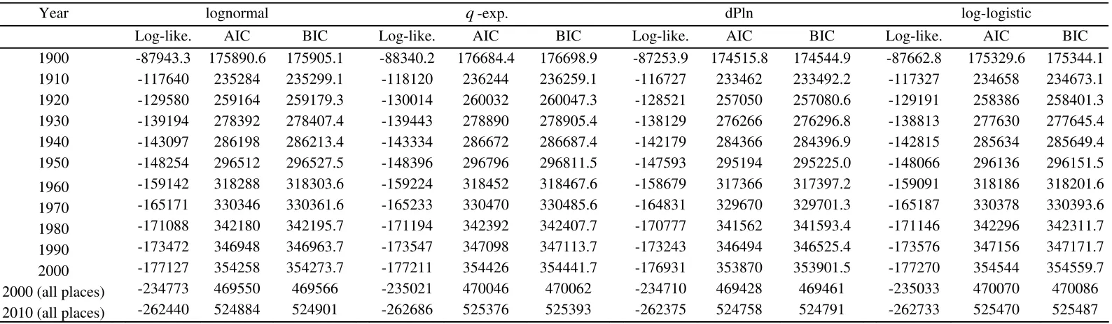
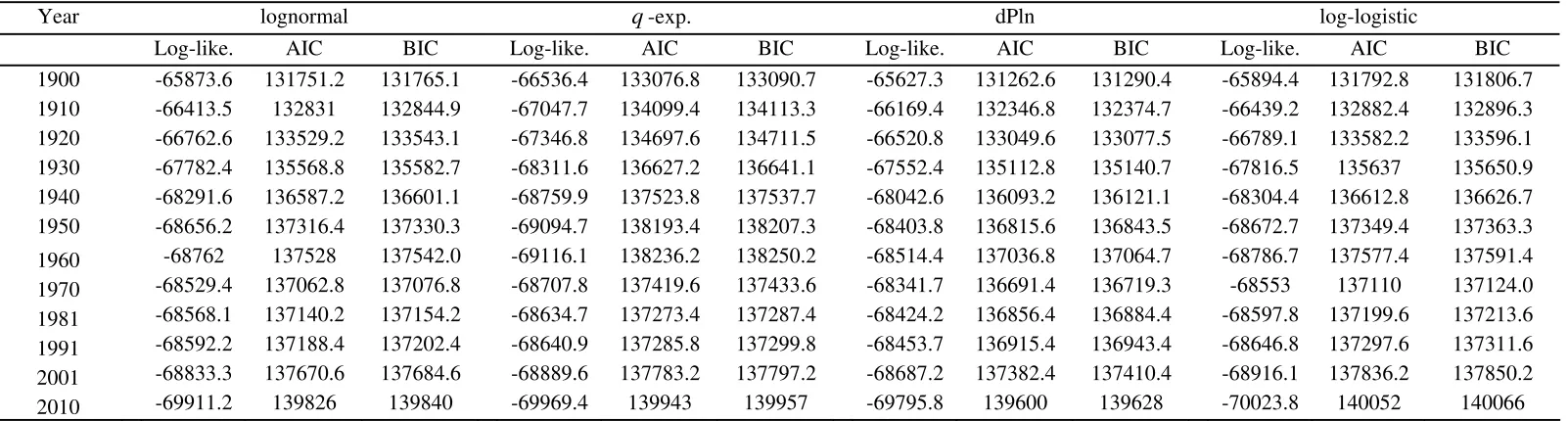
preferable to the BIC. From a long-term perspective (Tables 6, 7 and 8), there is always
agreement between the AIC and BIC, and the best distribution in all years in the US,
Spain and Italy is the dPln.
In short, if we consider all the evidence (cross-sectional and log-term) there are
68 cases: 13 periods for the US, 12 for Spain and Italy, and one for each of the rest of
the 31 OECD countries. In 62 of them there is a coincidence between the AIC and BIC
in the selection of the best fit. Therefore, out of the 68 cases, the dPln is the selected
model in 59 cases (86.76%), the ll in 7 cases (Belgium 2010, Chile 2002, Denmark
2012, Estonia 2012, Israel 2008, New Zealand 2006 and Slovenia 2012), the ln in one
case (Iceland 2012) and the qe also in one case (Korea 2012).
We wonder if there is any kind of geographic regularity in these results, but,
apparently, there is not. However, we have observed a certain relationship between
sample size and the best distribution for each country. When the sample size is below
106 cities (three cases) the dPln never provides the best fit. If the sample size is above
589 cities the dPln is always the selected distribution (51 cases). Finally, for between
106 and 589 cities the result is mixed: the dPln is the best distribution in 8 out of 14
cases. In short, there is a threshold in sample size (in our results around 600 cities)
above which the dPln clearly dominates; the only way that any of the other studied
distributions can be selected is if the sample size is low enough.9
5. Discussion
9
15 In this paper we compare four statistical distributions (the double Pareto lognormal, the
lognormal, the q-exponential and the log-logistic) used to fit the overall city size
distribution with un-truncated city size data. We combine a long-term perspective for
three countries (the US, Spain and Italy) with a long cross-sectional sample of countries
(the rest of the OECD countries).
A first important result is that the dPln is clearly in most of the cases and using
several criteria the best distribution out of the four studied. This result confirms the
conclusions obtained by Giesen et al. (2010) with a small sample of countries. It is a
reassuring result because it allows us to reconcile all the old literature about the validity
of the Pareto distribution (in the upper tail) and the particular case of Zipf´s law, with
more recent studies which raise doubts about its performance for the overall city size
distribution, and propose the lognormal as the most suitable distribution for
un-truncated city size data. There is indeed a new mainstream in the literature, to which we
contribute with this work, that argues that the best fit to un-truncated city size data is
provided by a mixture of Pareto and lognormal distributions, such as the dPln, which is
lognormal in the body and Pareto in the tails. In this line we can also include the
contribution by Ioannides and Skouras (2013), who have proposed a new statistical
distribution, but also combining lognormal and Pareto. It seems that the discussion
raised by Levy (2009) has been solved: “most cities obey a lognormal; but the upper tail
and therefore most of the population obeys a Pareto law” (Ioannides and Skouras,
2013).
Regarding the other distributions, out of the 68 cases studied, and according to
the AIC and BIC information criteria, the dPln is the best distribution in 59 of them
(86.76%), the ll in 7 (Belgium, Chile, Denmark, Estonia, Israel, New Zealand and
16 all the statistical information, we can rank in descending order the performance of the
distributions as follows: the dPln, the ll, the ln and finally the qe. It is surprising that a
newcomer distribution to urban economics, the log-logistic, appears in second place,
with the additional advantage of having a simpler functional form than the double
Pareto lognormal and two parameters instead of four.
With so many results and so much information, we wonder if there is any kind
of regularity that helps to explain the cases in which the dPln is the best or not. And we
find that the key issue is the sample size. We have detected that below a very small
sample size, in our data a lower bound around of 100 cities, the dPln is outperformed by
other distributions; however, above a certain threshold of the sample size, in our data
around 600 cities, the dPln clearly dominates the other studied distributions. For
intermediate sample sizes between 100 and 600 cities, the dPln is the best in roughly
half of the cases.
Finally, we would like to discuss a difficult and technical, but interesting, issue,
which is introduced in the theoretical model by Giesen and Suedekum (2012a): the
effect of age heterogeneity across cities on city size distribution. Giesen and Suedekum
(2012b) add empirical evidence relating to the cases of France and the US. Giesen and
Suedekum’s (2012a) theoretical model generates a dPln city size distribution based on
two basic features. Firstly, in each period new cities do enter at a constant rate.
Secondly, the age distribution of cities is heterogeneous. Both assumptions are different
from those of the theoretical model proposed by Eeckhout (2004), which yields to a
lognormal city size distribution. Focusing on the US, Spain and Italy (the three
countries we analyse from a temporal perspective), we find that the dPln is always
better than the ln although, according to the theoretical predictions, the relative edge
17 constant growth in the number of cities. In our results the dPln performs relatively better
than the ln in the US. In Spain and Italy the lognormal performs not so badly (the mean
AIC of the ln over the mean AIC of the dPln is 1.00401 for the US, 1.00298 for Spain
and 1.00172 for Italy). Is this result consistent with the theoretical model of Giesen and
Suedekum (2012a)? The answer to this question would require a detailed historical
study of the entry rate of cities and their age distribution in the three countries, a study
beyond the scope of this paper. We can only say that in our samples, considering the
whole twentieth century, there is city entry in the US, while in Spain and Italy the
number of cities remains almost constant. However, the age heterogeneity of the
European cities is much higher (the foundation of many European cities dates back to
the Middle Ages) than that of the United States (from 1600 to 2000 approximately). In
short, this is an open question deserving further research.
6. Conclusions
City size distribution has been the subject of numerous empirical investigations by
urban economists, statistical physicists, and urban geographers. From the point of view
of urban economics, the study of city size distribution has deep economic implications
related to labour markets, income distribution, public expenditure, etc.
Elsewhere, since the work of Eeckhout (2004), the risks of considering only the
largest cities have been demonstrated; that is, only the upper tail. In turn, if the
availability of data allows it, the analysis of city size distribution should be done as a
long-term analysis. With both considerations as premises, this article combines
un-truncated census data for the entire 20th century in decades, of three countries: the US,
Spain and Italy, with cross-sectional data from the most recent census of the rest of the
OECD countries. Using such comprehensives databases, with no size restriction, and
18 This work has minutely examined three density functions with relatively recent
use in urban economics, namely the lognormal, the q-exponential, the double Pareto
lognormal and an almost new distribution, the log-logistic. After estimating the
parameters of the four distributions by maximum likelihood, we have tested the fit
provided by each distribution using the Kolmogorov-Smirnov and Cramér-von Mises
tests. Afterwards, we have computed the AIC and BIC information criteria. Our results
show that, in general, the best function to describe city size distribution, out of the four
studied here, is the double Pareto lognormal.
Acknowledgements
The authors acknowledge financial support from the Spanish Ministerio de Educación y
Ciencia (ECO2009-09332 and ECO2010-16934 projects, and grant AP2008-03561), the
DGA (ADETRE research group), FEDER, and the Generalitat (2009SGR102). Earlier
versions of this paper were presented at the 59th Annual North American Meetings of
the Regional Science Association International (Ottawa, 2012) and at the XXXVII
Symposium of Economic Analysis (Vigo, 2012). All the comments made by
participants at these events were highly appreciated.
References
Anderson, G. and Y. Ge (2005). “The size distribution of Chinese cities,” Regional
Science and Urban Economics 35, 756–776.
Berry, B. J. L. and A. Okulicz-Kozaryn (2012). “The city size distribution debate:
Resolution for US urban regions and megalopolitan areas,” Cities 29, S17–S23.
Black, D. and J. V. Henderson (2003). “Urban evolution in the USA,” Journal of
19 Bosker, M., S. Brakman, H. Garretsen and M. Schramm (2008). “A century of shocks:
the evolution of the German city size distribution 1925–1999,” Regional Science and
Urban Economics 38, 330–347.
Burnham, K. P. and D. R. Anderson (2002). “Model selection and multimodel
inference: A practical information-theoretic approach.” Springer–Verlag.
Burnham, K. P. and D. R. Anderson (2004). “Multimodel inference: Understanding AIC
and BIC in model selection,” Sociological Methods and Research 33, 261-304.
Cameron, T. A. (1990). “One-stage structural models to explain city size,” Journal of
Urban Economics 27(3), 294–207.
Cheshire, P. (1999). “Trends in sizes and structure of urban areas,” in Handbook of
Regional and Urban Economics, Vol. 3, P. Cheshire and E. S. Mills (eds.) Amsterdam:
Elsevier Science, Chapter 35, 1339–1373.
Cheshire, P. C. and S. Magrini (2006). “Population growth in European cities: weather
matters-but only nationally,” Regional Studies 40(1), 23–37.
Choulakian, V. and M. A. Stephens (2001). “Goodness-of-fit tests for the generalized
Pareto distribution,” Technometrics 43, 478–484.
Eeckhout, J. (2004). “Gibrat’s Law for (all) cities,” American Economic Review 94(5),
1429–1451.
Fisk, P. R. (1961). “The graduation of income distributions,” Econometrica 29(2), 171–
185.
Gabaix, X. and Y. M. Ioannides (2004). “The evolution of city size distributions,” in
Handbook of Urban and Regional Economics, Vol. 4, J. V. Henderson and J. F. Thisse
20 Gibrat, R. (1931). “Les inégalités économiques,” Paris: Librairie du recueil Sirey.
Giesen, K. and J. Suedekum (2011). “Zipf´s law for cities in the regions and the
country,” Journal of Economic Geography 11, 667–686.
Giesen, K. and J. Suedekum (2012a). “The size distribution across all ‘cities’: A
unifying approach,” IEB Working Paper 2012/2.
Giesen, K. and J. Suedekum (2012b). “The French overall city size distribution,”
Région et Développement 36, 107–126.
Giesen, K., A. Zimmermann and J. Suedekum (2010). “The size distribution across all
cities – double Pareto lognormal strikes,” Journal of Urban Economics 68, 129–137.
González-Val, R. (2010). “The evolution of US city size distribution from a long term
perspective (1900–2000),” Journal of Regional Science 50, 952–972.
González-Val, R., L. Lanaspa and F. Sanz (2012). “New evidence on Gibrat’s law for
cities,” IEB Working Paper 2012/18.
Grimshaw, S. D. (1993). “Computing maximum likelihood estimates for the generalized
Pareto distribution,” Technometrics 35, 185–191.
Hosking, J. R. M. and J. R. Wallis (1987). “Parameter and quantile estimation for the
generalized Pareto distribution,” Technometrics 29, 339–349.
Hsing, Y. (1990). “A note on functional forms and the urban size distribution,” Journal
of Urban Economics 27(1), 73–79.
Hsu, W.-T. (2012). “Central place theory and city size distribution,” The Economic
Journal 122, 903–932.
Ioannides, Y. M. and H. G. Overman (2003). “Zipf’s law for cities: an empirical
21 Ioannides, Y. M. and S. Skouras (2013). “US city size distribution: Robustly Pareto, but
only in the tail,” Journal of Urban Economics 73, 18–29.
Kalecki, M. (1945). “On the Gibrat distribution,” Econometrica 13(2), 161–170.
Kamecke, U. (1990). “Testing the rank size rule hypothesis with an efficient estimator,”
Journal of Urban Economics 27(2), 222–231.
Levy, M. (2009). “Gibrat´s Law for (All) Cities: Comment,” American Economic
Review 99, 1672–1675.
Malacarne, L. C., R. S. Mendes and E. K. Lenzi (2001). “q-exponential distribution in
urban agglomeration,” Physical Review E 65(017106), 1–3.
Michaels, G., F. Rauch and S. J. Redding (2012). “Urbanization and structural
transformation,” The Quarterly Journal of Economics 127(2), 535–586.
Pareto, V. (1896). “Cours d’économie politique,” Geneva: Droz.
Parr, J. B. and K. Suzuki (1973). “Settlement populations and the lognormal
distribution,” Urban Studies 10, 335–352.
Razali, N.M. and Y.B. Wah (2011). “Power comparisons of Shapiro-Wilk,
Kolmogorov-Smirnov, Lilliefors and Anderson-Darling tests,” Journal of Statistical
Modeling and Analytics 2, 21–33.
Reed, W. (2001). “The Pareto, Zipf and other power laws,” Economics Letters 74, 15–
19.
Reed, W. (2002). “On the rank-size distribution for human settlements,” Journal of
22 Reed, W. and M. Jorgensen (2004). “The double Pareto-lognormal distribution – A new
parametric model for size distribution,” Com. Stats. –Theory & Methods 33, 1733–
1753.
Richardson, H. W. (1973). “Theory of the distribution of city sizes: Review and
prospects,” Regional Studies 7, 239–251.
Rosen, K. and M. Resnick (1980). “The size distribution of cities: an examination of the
Pareto law and primacy,” Journal of Urban Economics 8, 165–186.
Rozenfeld, H. D., D. Rybski, X. Gabaix and H. A. Makse (2011). “The Area and
Population of Cities: New Insights from a Different Perspective on Cities,” American
Economic Review 101(5), 2205–25.
Shalizi, C. (2007). “Maximum likelihood estimation for q-exponential (Tsallis)
Distributions,” arXiv: math/0701854v2.
Singh, S. K. and G. S. Maddala (2008). “A function for size distribution of incomes,” in
Modeling Income Distributions and Lorenz Curves. Economic Studies in Inequality,
Social Exclusion and Well-Being, Volume 5, I, 27–35.
Soo, K. T. (2005). “Zipf’s Law for cities: a cross-country investigation,” Regional
Science and Urban Economics 35, 239–263.
Soo, K. T. (2007). “Zipf's Law and urban growth in Malaysia,” Urban Studies 44(1), 1–
14.
Tsallis, C. (1988). “Possible generalization of Boltzmann-Gibbs statistics,” Journal of
Statistical Physics 52, 479–487.
Zipf, G. K. (1949). “Human behaviour and the principle of least effort,” Cambridge,
23 Table 1. Number of cities and descriptive statistics: the US, Spain and Italy
US
Year Cities Mean
Standard
deviation Minimum Maximum
1900 10,596 3,376.04 42,323.90 7 3,437,202
1910 14,135 3,560.92 49,351.24 4 4,766,883
1920 15,481 4,014.81 56,781.65 3 5,620,048
1930 16,475 4,642.02 67,853.65 1 6,930,446
1940 16,729 4,975.67 71,299.37 1 7,454,995
1950 17,113 5,613.42 76,064.40 1 7,891,957
1960 18,051 6,408.75 74,737.62 1 7,781,984
1970 18,488 7,094.29 75,319.59 3 7,894,862
1980 18,923 7,395.64 69,167.91 2 7,071,639
1990 19,120 7,977.63 71,873.91 2 7,322,564
2000 19,296 8,968.44 78,014.75 1 8,008,278
2000 (all places) 25,358 8,231.53 68,390.23 1 8,008,278
2010 (all places) 28,664 7,871.53 61,631.70 1 8,175,133
Spain
Year Cities Mean
Standard
deviation Minimum Maximum
1900 7,800 2,282.40 10,177.75 78 539,835
1910 7,806 2,452.01 11,217.02 92 599,807
1920 7,812 2,621.92 13,501.02 82 750,896
1930 7,875 2,892.18 17,513.90 79 1,005,565
1940 7,896 3,180.65 20,099.96 11 1,088,647
1950 7,901 3,479.86 26,033.29 64 1,618,435
1960 7,910 3,801.71 33,652.11 51 2,259,931
1970 7,956 4,240.98 43,971.93 10 3,146,071
1981 8,034 4,701.40 45,995.35 5 3,188,297
1991 8,077 4,882.27 45,219.85 2 3,084,673
2001 8,077 5,039.37 43,079.46 7 2,938,723
2010 8,114 7,795.05 47,529.80 5 3,273,049
Italy
Year Cities Mean
Standard
deviation Minimum Maximum
1901 7,711 4,274.84 14,424.61 56 621,213
1911 7,711 4,648.11 17,392.98 58 751,211
1921 8,100 4,863.80 20,031.61 58 859,629
1931 8,100 5,067.10 22,559.85 93 960,660
1936 8,100 5,234.38 25,274.48 116 1,150,338
1951 8,100 5,866.12 31,137.52 74 1,651,393
1961 8,100 6,249.82 39,130.55 90 2,187,682
1971 8,100 6,683.52 45,581.66 51 2,781,385
1981 8,100 6,982.33 45,329.33 32 2,839,638
1991 8,100 7,009.63 42,450.26 31 2,775,250
2001 8,100 7,021.20 39,325.47 33 2,546,804
2010 8,094 7,490.29 41,505.4 34 2,761,477
24 Table 2. Number of cities and descriptive statistics: Rest of the OECD countries
Country Year Cities Mean
Standard
deviation Minimum Maximum
Australia 2001 1,559 10,756.6 132,419 200 3,502,301
Austria 2001 2,359 3,405.23 32,855.2 60 1,550,123
Belgium 2010 589 18,403.9 29,353.6 80 483,505
Canada 2011 4,931 6,789.03 57,345.8 5 2,615,060
Chile 2002 342 44,200.1 68,452 130 492,915
Czech Republic 2011 6,251 1,684.97 17,825 3 1,257,158
Denmark 2012 99 56,435.2 65,246.2 104 551,900
Estonia 2012 232 23,108.3 129,319 67 1,339,662
Finland 2011 335 16,062.5 42,665.6 103 595,384
France 2009 36,716 1,790.92 8,253.09 1 447,396
Germany 2010 11,292 7,239.78 46,688.7 8 3,460,725
Greece 2011 325 33,187.3 49,804.8 150 655,780
Hungary 2001 3,121 3,245.99 33,161.7 12 1,777,921
Iceland 2012 75 4,261 14,446.2 52 118,814
Ireland 2011 824 3,850.91 39,696.9 90 1,110,627
Israel 2008 169 39,203.6 76,876.4 5000 759,700
Japan 2010 2,102 25,863 74,416.4 140 1,468,382
Korea 2012 251 191,198 149,616 7,737 640,732
Luxemburg 2012 106 4,951.44 10,370.9 677 99,852
Mexico 2010 2,456 45,092.8 130,512 93 1,794,969
Netherlands 2001 504 31,717.3 54,134.7 1,017 734,533
New Zealand 2006 74 54,431.8 75,920.8 417 404,658
Norway 2012 429 11,622.1 35,497.4 218 613,285
Poland 2010 2,479 15,409.5 50,664 1,361 1,720,398
Portugal 2011 308 34,291 56,055.8 430 547,631
Slovakia 2001 2,926 1,844.51 5,857.66 8 105,842
Slovenia 2012 211 9,741.69 21,846.4 379 280,607
Sweden 2010 290 32,442.5 64,826.9 2,446 845,777
Switzerland 2010 2,495 3,154.36 10,879.7 12 372,857
Turkey 2011 2,934 21,362.9 75,364.6 328 831,229
25 Table 3. Estimated parameters of the distributions
Lognormal distribution
q-exponential distribution
Log-logistic distribution
Double Pareto lognormal distribution
Country Year μ σ q a μ σ α β μ σ
Australia 2001 7.04 1.33 1.75 0.0016 6.88 0.70 0.66 24.89 5.57 0.21
Austria 2001 7.39 0.89 1.22 0.0006 7.37 0.48 1.59 1.98 7.27 0.37
Belgium 2010 9.39 0.87 1.14 0.0001 9.38 0.47 1.85 2.26 9.30 0.50
Canada 2011 6.66 1.86 2.05 0.0027 6.65 1.01 0.78 0.82 6.60 0.69
Chile 2002 9.82 1.38 1.53 0.0001 9.82 0.77 2.89 1.42 10.18 1.14
Czech Republic 2011 6.15 1.22 1.56 0.0030 6.07 0.67 1.07 4.72 5.43 0.77
Denmark 2012 10.58 0.99 1.05 1.9e-5 10.66 0.43 -- -- -- --
Estonia 2012 7.84 1.33 1.73 0.0007 7.69 0.63 -- -- -- --
Finland 2011 8.78 1.21 1.49 0.0002 8.72 0.67 1.10 1.82 8.41 0.62
France 2009 6.21 1.35 1.67 0.0031 6.14 0.75 1.00 3.32 5.52 0.88
Germany 2010 7.52 1.51 1.77 0.0009 7.49 0.87 1.34 3.73 7.04 1.29
Greece 2011 9.73 1.34 1.19 4.5e-5 9.84 0.72 2.46 0.88 10.46 0.60
Hungary 2001 6.82 1.30 1.56 0.0015 6.78 0.72 1.18 2.05 6.47 0.86
Iceland 2012 6.85 1.59 1.89 0.0020 6.79 0.90 1.00 3.93 6.10 1.21
Ireland 2011 6.64 1.29 1.72 0.0023 6.49 0.69 0.76 13.91 5.39 0.37
Israel 2008 9.89 1.03 1.38 0.0001 9.80 0.58 -- -- -- --
Italy 2010 7.85 1.34 1.55 0.0005 7.83 0.76 1.58 3.65 7.49 1.15
Japan 2010 9.14 1.24 1.56 1.4e-4 9.07 0.68 0.99 1.69 8.72 0.48
Korea 2012 11.76 0.98 0.62 2.3e-6 11.82 0.59 7.06 1.43 12.32 0.73
Luxemburg 2012 7.96 0.88 1.25 0.0004 7.89 0.48 1.22 12.45 7.22 0.41
Mexico 2010 9.41 1.55 1.77 0.0001 9.40 0.88 1.41 3.26 9.01 1.35
Netherlands 2001 9.91 0.85 1.18 4.6e-5 9.86 0.47 1.52 2.78 9.61 0.42
New Zealand 2006 10.25 1.22 1.27 3.2e-5 10.29 0.66 1.55 1.17 10.46 0.58
Norway 2012 8.50 1.17 1.44 0.0002 8.45 0.66 1.29 5.66 7.90 0.86
Poland 2010 9.07 0.82 1.25 0.0001 8.99 0.43 1.36 9.10 8.44 0.35
Portugal 2011 9.73 1.14 1.40 0.0001 9.67 0.66 1.25 5.47 9.11 0.82
Slovakia 2001 6.54 1.20 1.48 0.0018 6.50 0.65 1.21 1.77 6.27 0.64
Slovenia 2012 8.58 0.99 1.26 0.0002 8.55 0.55 1.50 2.37 8.34 0.60
Spain 2010 6.58 1.85 2.29 0.0041 6.49 1.07 0.75 3.84 5.52 1.31
Sweden 2010 9.82 0.94 1.25 0.0001 9.76 0.53 1.33 8.58 9.19 0.59
Switzerland 2010 7.11 1.32 1.48 0.0010 7.10 0.75 1.93 2.44 7.00 1.14
Turkey 2011 8.27 1.44 1.92 0.0006 8.06 0.74 0.75 3.59 7.21 0.34
United Kingdom 2001 11.68 0.59 -- -- 11.67 0.31 2.24 2.94 11.57 0.16
US 2010 7.13 1.83 2.17 0.0020 7.09 1.05 1.17 2.97 6.61 1.59
26 Table 4. p-values of the Kolmogorov-Smirnov (KS) and Cramér-von Mises (CM) tests
Notes: The null hypothesis is that the empirical distribution follows the lognormal,
q
-exponential, dPln or log-logistic distribution. The cases in which the statistical distribution cannot be rejected at the 5% significance level are highlighted in bold. It has not been possible to perform the tests for the dPln distribution for Australia (2001), Denmark (2012), Estonia (2012), Israel (2008), Luxembourg (2012), Poland (2010) and Sweden (2010), and for the qe distribution for the UK (2001). In these few cases, we could not generate the samples with which the test are performed in the same way as in the other cases. The reason seems to be the extremely flat lower tail in these cases.Lognormal distribution q-exponential distribution Double Pareto lognormal distribution Log-logistic distribution
KS CM KS CM KS CM KS CM
Australia 2001 0 0 0 0 - - 0 0
Austria 2001 0 0 0 0 0.854 0.809 0.181 0.164 Belgium 2010 0.382 0.224 0 0 0.993 0.985 0.998 0.993 Canada 2011 0 0 0.006 0.017 0.112 0.187 0.002 0.011
Chile 2002 0.172 0.131 0 0 0.094 0.118 0.249 0.247 Czech Republic 2011 0 0 0 0 0.173 0.362 0 0.007
Denmark 2012 0 0 0 0 - - 0.434 0.266 Estonia 2012 0.002 0 0 0 - - 0.045 0.619 Finland 2011 0.134 0.177 0.002 0.015 0.963 0.970 0.736 0.619
France 2009 0 0 0 0 0.046 0.070 0 0
Germany 2010 0 0 0 0 0.002 0.008 0 0
Greece 2011 0.001 0.009 0.172 0.376 0.706 0.766 0.300 0.259 Hungary 2001 0.002 0.005 0 0 0.682 0.653 0.134 0.193 Iceland 2012 0.855 0.932 0.959 0.980 0.987 0.992 0.979 0.991 Ireland 2011 0 0 0 0 0.397 0.456 0 0
Israel 2008 0.093 0.128 0 0 - - 0.060 0.276 Italy 2010 0.096 0.062 0 0 0.978 0.942 0.016 0.017 Japan 2010 0 0 0 0 0.435 0.483 0.027 0.009 Korea 2012 0 0.003 0.043 0.096 0.002 0.008 0 0.002 Luxemburg 2012 0.289 0.322 0 0.007 - - 0.662 0.617
Mexico 2010 0.243 0.246 0 0 0.168 0.210 0.151 0.141 Netherlands 2001 0.043 0.044 0 0 0.896 0.913 0.532 0.518 New Zealand 2006 0.778 0.591 0.372 0.458 0.668 0.870 0.670 0.850 Norway 2012 0.310 0.236 0 0 0.842 0.851 0.465 0.388
Poland 2010 0 0 0 0 - - 0 0
Portugal 2011 0.244 0.111 0 0 0.373 0.384 0.364 0.179 Slovakia 2001 0 0 0 0 0.670 0.584 0.495 0.534 Slovenia 2012 0.502 0.385 0 0.006 0.860 0.847 0.692 0.541
Spain 2010 0 0 0 0 0 0 0 0
Sweden 2010 0.015 0.066 0 0 - - 0.094 0.160 Switzerland 2010 0.819 0.930 0 0 0.809 0.959 0.162 0.259
Turkey 2011 0 0 0 0 0.001 0.005 0 0
United Kingdom 2001 0.016 0.049 - - 0.500 0.476 0.385 0.257
27 Table 5. Results of the information criteria: Rest of the OECD countries
lognormal q-exp. dPln log-logistic
Country Log-like. AIC BIC Log-like. AIC BIC Log-like. AIC BIC Log-like. AIC BIC
Australia -13635.8 27276 27286 -13667.3 27339 27349 -13374.3 26757 26778 -13568.7 27141 27152
Austria -20516.7 41037 41049 -20807.5 41619 41631 -20415.5 40839 40862 -20429.7 40863 40875
Belgium -6282.8 12570 12578 -6377.9 12760 12768 -6267 12542 12560 -6268 12540 12549
Canada -42872.2 85748 85761 -42784 85572 85585 -42772.8 85554 85580 -42784.7 85573 85586
Chile -3955.8 7916 7923 -3972.5 7949 7957 -3953.8 7916 7931 -3954.2 7912 7920
Czech Republic -48577.4 97159 97172 -48852.3 97709 97172 -48284.2 96576 96603 -48451 96906 96916
Denmark -1187.1 2378 2383 -1181.8 2368 2373 -- -- -- -11.68.4 2341 2346
Estonia -2215.1 4434 4441 -2211.3 4427 4433 -- -- -- -2185.6 4375 4382
Finland -3480.2 6964 6972 -3494.1 6992 7000 -3472.3 6953 6968 -3475.7 6955 6963
France -291228 582460 582477 -292189 584382 584399 -290114 580236 580270 -290877 581758 581775
Germany -105632 211268 211283 -105818 211640 211655 -105586 211180 211209 -105736 211476 211491
Greece -3717.3 7439 7446 -3697.1 7398 7406 -3694.9 7398 7413 -3709.1 7422 7430
Hungary -26540.9 53086 53098 -26619.5 53243 53255 -26482.7 52973 52998 -26504.3 53013 53025
Iceland -654.6 1313 1318 -655.3 1315 1319 -653.7 1315 1325 -654.8 1314 1318
Ireland -6851.8 13708 13717 -6885.4 13775 13784 -6726.6 13461 13480 -6829.2 13662 13672
Israel -1915.9 3836 3842 -1948.5 3901 3907 -- -- -- -1915.9 3836 3842
Japan -22651.3 45307 45318 -22735 45474 45485 -22567.4 45143 45165 -22607.8 45220 45231
Korea -3304.08 6612 6619 -3290.3 6585 6592 -3303.7 6615 6630 -3314.3 6633 6640
Luxemburg -980.4 1965 1970 -997.3 1999 2004 -972.4 1953 1963 -978.7 1961 1967
Mexico -27675.1 55354 55366 -27730.3 55465 55476 -27669.6 55347 55370 -27684.9 55374 55385
Netherlands -5629.3 11263 11271 -5703.1 11410 11419 -5609.8 11228 11245 -5617.9 11240 11248
28 Table 5. Results of the information criteria: Rest of the OECD countries – Continued
lognormal q-exp. dPln log-logistic
Country Log-like. AIC BIC Log-like. AIC BIC Log-like. AIC BIC Log-like. AIC BIC
Norway -4320.1 8644 8652 -4348.8 8702 8710 -4312.6 8633 8649 -4321.4 8647 8655
Poland -25511.7 51027 51039 -26012.2 52028 52040 -25212.4 50433 50456 -25392 50788 50800
Portugal -3473.8 6952 6959 -3509.1 7022 7030 -3470.6 6949 6964 -3477.8 6960 6967
Slovakia -23804.8 47614 47626 -23921.8 47848 47860 -23712.7 47433 47457 -23732.9 47470 47482
Slovenia -2107.6 4219 4226 -2126.8 4258 4264 -2104.1 4216 4230 -2105.4 4215 4222
Sweden -3242.6 6489 6497 -3319.2 6642 6650 -3233 6474 6489 -3242 6488 6495
Switzerland -21958.3 43921 43932 -22008.4 44021 44032 -21955.4 43919 43942 -21971.1 43946 43958
Turkey -29486.3 58977 58989 -29492.4 58989 59001 -28876.7 57761 57785 -29330.6 58665 58677
United Kingdom -4448.1 8900 8908 -- -- -- -4424.8 8858 8873 -4426.9 8858 8866
Note: The Akaike Information Criterion for distribution i is computed as AICi =2⋅ki −2⋅ln
( )
Li and the Schwarz Criterion as( )
( )
ii
i k N L
29 Table 6. Results of the information criteria: the US
Year lognormal q-exp. dPln log-logistic
Log-like. AIC BIC Log-like. AIC BIC Log-like. AIC BIC Log-like. AIC BIC
1900 -87943.3 175890.6 175905.1 -88340.2 176684.4 176698.9 -87253.9 174515.8 174544.9 -87662.8 175329.6 175344.1
1910 -117640 235284 235299.1 -118120 236244 236259.1 -116727 233462 233492.2 -117327 234658 234673.1
1920 -129580 259164 259179.3 -130014 260032 260047.3 -128521 257050 257080.6 -129191 258386 258401.3
1930 -139194 278392 278407.4 -139443 278890 278905.4 -138129 276266 276296.8 -138813 277630 277645.4
1940 -143097 286198 286213.4 -143334 286672 286687.4 -142179 284366 284396.9 -142815 285634 285649.4
1950 -148254 296512 296527.5 -148396 296796 296811.5 -147593 295194 295225.0 -148066 296136 296151.5
1960 -159142 318288 318303.6 -159224 318452 318467.6 -158679 317366 317397.2 -159091 318186 318201.6
1970 -165171 330346 330361.6 -165233 330470 330485.6 -164831 329670 329701.3 -165187 330378 330393.6
1980 -171088 342180 342195.7 -171194 342392 342407.7 -170777 341562 341593.4 -171146 342296 342311.7
1990 -173472 346948 346963.7 -173547 347098 347113.7 -173243 346494 346525.4 -173576 347156 347171.7
2000 -177127 354258 354273.7 -177211 354426 354441.7 -176931 353870 353901.5 -177270 354544 354559.7
2000 (all places) -234773 469550 469566 -235021 470046 470062 -234710 469428 469461 -235033 470070 470086
2010 (all places) -262440 524884 524901 -262686 525376 525393 -262375 524758 524791 -262733 525470 525487
Note: The Akaike Information Criterion for distribution i is computed as AICi =2⋅ki −2⋅ln
( )
Li and the Schwarz Criterion as( )
( )
ii
i k N L
30 Table 7. Results of the information criteria: Spain
Year lognormal q-exp. dPln log-logistic
Log-like. AIC BIC Log-like. AIC BIC Log-like. AIC BIC Log-like. AIC BIC
1900 -65873.6 131751.2 131765.1 -66536.4 133076.8 133090.7 -65627.3 131262.6 131290.4 -65894.4 131792.8 131806.7
1910 -66413.5 132831 132844.9 -67047.7 134099.4 134113.3 -66169.4 132346.8 132374.7 -66439.2 132882.4 132896.3
1920 -66762.6 133529.2 133543.1 -67346.8 134697.6 134711.5 -66520.8 133049.6 133077.5 -66789.1 133582.2 133596.1
1930 -67782.4 135568.8 135582.7 -68311.6 136627.2 136641.1 -67552.4 135112.8 135140.7 -67816.5 135637 135650.9
1940 -68291.6 136587.2 136601.1 -68759.9 137523.8 137537.7 -68042.6 136093.2 136121.1 -68304.4 136612.8 136626.7
1950 -68656.2 137316.4 137330.3 -69094.7 138193.4 138207.3 -68403.8 136815.6 136843.5 -68672.7 137349.4 137363.3
1960 -68762 137528 137542.0 -69116.1 138236.2 138250.2 -68514.4 137036.8 137064.7 -68786.7 137577.4 137591.4
1970 -68529.4 137062.8 137076.8 -68707.8 137419.6 137433.6 -68341.7 136691.4 136719.3 -68553 137110 137124.0
1981 -68568.1 137140.2 137154.2 -68634.7 137273.4 137287.4 -68424.2 136856.4 136884.4 -68597.8 137199.6 137213.6
1991 -68592.2 137188.4 137202.4 -68640.9 137285.8 137299.8 -68453.7 136915.4 136943.4 -68646.8 137297.6 137311.6
2001 -68833.3 137670.6 137684.6 -68889.6 137783.2 137797.2 -68687.2 137382.4 137410.4 -68916.1 137836.2 137850.2
2010 -69911.2 139826 139840 -69969.4 139943 139957 -69795.8 139600 139628 -70023.8 140052 140066
Note: The Akaike Information Criterion for distribution i is computed as AICi =2⋅ki −2⋅ln
( )
Li and the Schwarz Criterion as( )
( )
i ii k N L
BIC = ⋅ln −2⋅ln , where ki is the number of free parameters of distribution i, N is the number cities by year, and ln
( )
Li is the31 Table 8. Results of the information criteria: Italy
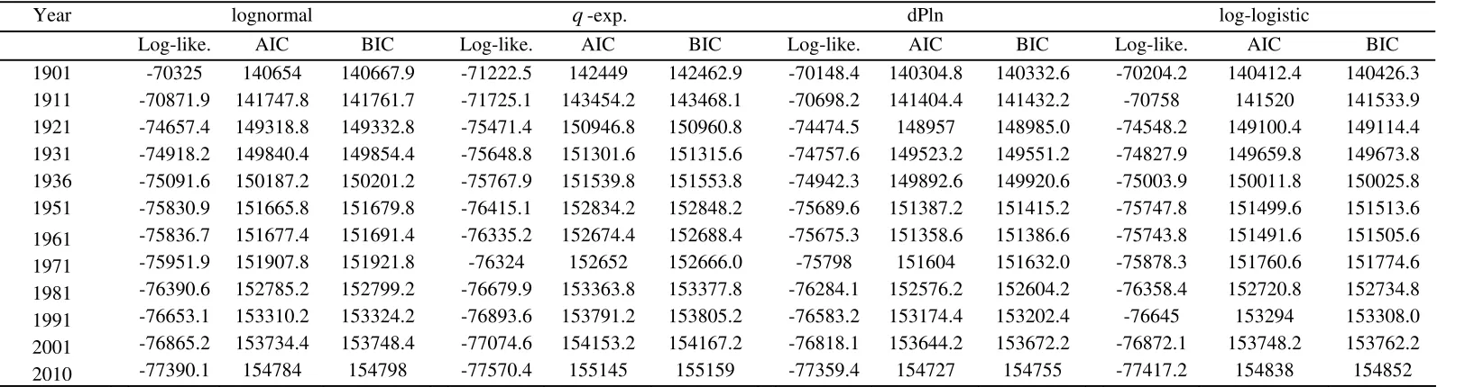
Year lognormal q-exp. dPln log-logistic
Log-like. AIC BIC Log-like. AIC BIC Log-like. AIC BIC Log-like. AIC BIC
1901 -70325 140654 140667.9 -71222.5 142449 142462.9 -70148.4 140304.8 140332.6 -70204.2 140412.4 140426.3
1911 -70871.9 141747.8 141761.7 -71725.1 143454.2 143468.1 -70698.2 141404.4 141432.2 -70758 141520 141533.9
1921 -74657.4 149318.8 149332.8 -75471.4 150946.8 150960.8 -74474.5 148957 148985.0 -74548.2 149100.4 149114.4
1931 -74918.2 149840.4 149854.4 -75648.8 151301.6 151315.6 -74757.6 149523.2 149551.2 -74827.9 149659.8 149673.8
1936 -75091.6 150187.2 150201.2 -75767.9 151539.8 151553.8 -74942.3 149892.6 149920.6 -75003.9 150011.8 150025.8
1951 -75830.9 151665.8 151679.8 -76415.1 152834.2 152848.2 -75689.6 151387.2 151415.2 -75747.8 151499.6 151513.6
1961 -75836.7 151677.4 151691.4 -76335.2 152674.4 152688.4 -75675.3 151358.6 151386.6 -75743.8 151491.6 151505.6
1971 -75951.9 151907.8 151921.8 -76324 152652 152666.0 -75798 151604 151632.0 -75878.3 151760.6 151774.6
1981 -76390.6 152785.2 152799.2 -76679.9 153363.8 153377.8 -76284.1 152576.2 152604.2 -76358.4 152720.8 152734.8
1991 -76653.1 153310.2 153324.2 -76893.6 153791.2 153805.2 -76583.2 153174.4 153202.4 -76645 153294 153308.0
2001 -76865.2 153734.4 153748.4 -77074.6 154153.2 154167.2 -76818.1 153644.2 153672.2 -76872.1 153748.2 153762.2
2010 -77390.1 154784 154798 -77570.4 155145 155159 -77359.4 154727 154755 -77417.2 154838 154852
Note: The Akaike Information Criterion for distribution i is computed as AICi =2⋅ki −2⋅ln
( )
Li and the Schwarz Criterion as( )
( )
i ii k N L
BIC = ⋅ln −2⋅ln , where ki is the number of free parameters of distribution i, N is the number cities by year, and ln
( )
Li is the32 Figure 1. Empirical and estimated pdfs in the US, Spain and Italy (2010)
0 .05 .1 .15 .2 .25 Density
0 5 10 15
Population (ln scale)
Empirical p.d.f. dPln log-logistic
lognormal q-exponential US 2010 Estimated p.d.f.
0 .02 .04 .06 .08 Density
10 12 14 16
Population (ln scale)
Empirical p.d.f. dPln log-logistic
lognormal q-exponential US 2010 Estimated p.d.f. (Zoom upper-tail)
0 .05 .1 .15 .2 .25 Density
0 5 10 15
Population (ln scale)
Empirical p.d.f. dPln log-logistic
lognormal q-exponential Spain 2010 Estimated p.d.f.
0 .01 .02 .03 .04 .05 Density
10 11 12 13 14 15
Population (ln scale)
Empirical p.d.f. dPln log-logistic
lognormal q-exponential Spain 2010 Estimated p.d.f. (Zoom upper-tail)
0 .1 .2 .3 .4 Density
3 6 9 12 15
Population (ln scale)
Empirical p.d.f. dPln log-logistic
lognormal q-exponential Italy 2010 Estimated p.d.f.
0 .02 .04 .06 .08 Density
10 11 12 13 14 15
Population (ln scale)
Empirical p.d.f. dPln log-logistic