2017 2nd International Conference on Computer Science and Technology (CST 2017) ISBN: 978-1-60595-461-5
Research on Aggregations for Algebraic Multigrid
Preconditioning Methods
Jian-ping WU
1,a*, Fu-kang YIN
1, Jun PENG
1and Jin-hui YANG
11 Academy of Ocean Science and Engineering, National University of Defense
Technology, Changsha, China
*Corresponding author
Keywords: Sparse linear system, Aggregation based algebraic multigrid, Smoothing process, Preconditioner, Krylov subspace method.
Abstract. Aggregation based algebraic multigrid is one of the most efficient methods to solve sparse linear systems. In this paper, a new method based on cliques and several classical aggregations are implemented based on sparse data structures, and compared in solving sparse linear systems from model partial differential equations. The results show that with Vanek scheme, the number of levels is often less than that with others, and when Jacobi smoothing is used, the number of preconditioned iterations and the time elapsed for iteration are both the least, while the time for setup is too long. From the view point of strong connections, it is beneficial to aggregate the points in a common clique, but the experiments have not shown this privilege. Instead, the two-point aggregation based on strong connection is effective in most cases, and the four-point and the eight-point aggregations which are based on loop of the two-point algorithm with two or three times respectively are effective too. In respect to total computation time, the best scheme is always one of these three schemes. In addition, the larger the average degree the related adjacent graph has, the less time required for the Vanek scheme to setup is and the more efficient it is, so is the aggregation scheme based on cliques.
Introduction
Multigrid is an efficient method to solve sparse linear systems, and is often combined with Krylov subspace iterations to improve the robustness [1]. The multigrid method is composed of two processes, smoothing and correction, which are used to reduce the error components with higher and lower frequencies respectively [2]. When smoothing is given, the more accurate the approximation of the linear system on the coarser grid to that on the finer is, and the more accurate the transfer operator is, the more effective the method will be.
Algebraic multigrid is used for general purpose [3] and the aggregation-type is one of the most favorite, for its cheap cost in both computation and storage [4]. In this kind of method, several points are related to a point on the coarser grid, which are called an aggregation. The selection of aggregation is the core in aggregation-type multigrid and it is often selected based on the adjacent graph.
pair-wise matching followed by another [4], with which the grid complexity on the coarser grid is reduced to about 1/4 to that on the finer.
Aggregations can also be selected based on the concept of strong connection. Braess provide a method to aggregate approximately four points once a time [7], which is composed of two steps. Vanek provide another algorithm depending on the concept of strongly coupling [8], where the isolated points are aggregated into an existed subset as soon as possible.
In this paper, a new aggregation method based on clique is provided and some classical methods are implemented with sparse data structures and then compared when combined with Jacobi and Gauss-Seidel smoothing. The results show that the Vanek scheme has potential to reduce the number of levels and the number of preconditioned iterations, and the best effective scheme is always the two-point aggregation or one of its versions with loop of several times.
Conjugate Gradient Preconditioned by Aggregation Based Algebraic Multigrid Consider the following linear system of order n
A x = b. (1) where A is a symmetric positive definite sparse matrix, b is a known vector, and x is the unknown solution. The details of the preconditioned conjugate gradient (PCG) method can be referred to algorithm 9.1 in [9], where M-1 is the so-called preconditioner.
In this paper, the aggregation based algebraic multigrid is used as the preconditioner, which is one class of multigrid methods (MGM). Its details can be referred to algorithm 2.3.2 in [10]. We adopt the V cycle with only 1 pre- and post- smoothing respectively. The pre- and the post- smoothing operator can be different and denoted as SlR and SlL respectively. During the coarsening, if the number of levels attains the threshold, or the sparse linear system is small enough, the process is stopped. The solution on the coarsest level is performed with ILU(0) preconditioned PCG iterations [9].
In algebraic multigrid, the interpolator is a matrix, with the number of rows and columns equal to the number of grid-points on the finer and coarser level respectively. For aggregation based algebraic multigrid preconditioner, we exploit the simplest interpolator. If a grid-point k on the finer level is related to a grid-point j on the coarser level, the entry at row k and column j is 1. All other entries not equal to 1 are set to zero. To ensure the symmetry of multigrid, we can select the restrictor as the transpose of the interpolator, and SL=(SR)T. In this way, the reduced linear system on the coarser level is determined. Then, to apply MGM, the remaining work is to select the coarser grid, and the smoother SlR on the finer grid.
When solving sparse linear systems with the multigrid preconditioned iterations, the grid hierarchy, the coefficient matrix, the grid transfer operator, and the smoother are all not changed during the iterative process. Therefore, they can be determined during the setup, and be reused directly in the latter iterations.
Classical Aggregation Algorithms
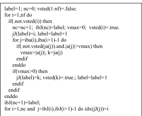
related element in the coefficient matrix. If there are no such nodes, it is itself regarded as an aggregation. This process is continued, until all nodes are aggregated. This scheme is denoted as aggst in this paper and can be described as in figure 1.
Figure 1. The aggregation algorithm based on strongest connection.
In figure 1, the coefficient matrix on the current level is stored in a, iba and ja in CSR format. The signs nf and nc mean the number of points in the current and the coarser level respectively. At the end of the algorithm, the grid-points in the current level are aggregated into nc sets, and the points of the i-th aggregation are stored in jJ(ibJ(i)) to jJ(ibJ(i+1)-1). For a grid-point k in the current level, idx(k) denotes the related grid-point in the coarser level.
Algorithm aggst can be used several times repeatedly to reduce the number of levels [4][6]. If two times used each time, we denote the related algorithm as agg4p and the number of grid-points on each level is reduced to about 1/4 of that on the finer. If three times used each time, we denote the related algorithm as agg8p and the number of grid-points on each level is reduced to about 1/8 of that on the finer.
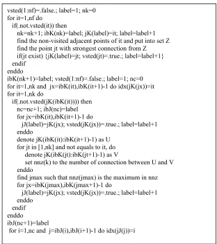
In Braess algorithm, approximately four points are aggregated once a time [7]. In this method, every two strongly connected points are matched and put into a subset. Each unmatched point is put into a subset alone. Then, every two subsets with maximum number of connections are aggregated. This scheme is denoted as aggbr in this paper and the details can be described as in figure 2.
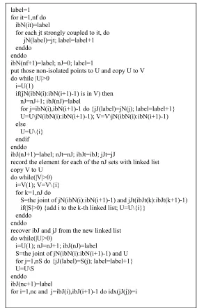
Vanek algorithm consists of four steps [8]. First the non-isolated points are recorded and the isolated ones will not belong to any aggregation. Secondly, the rest non-isolated points whose adjacent and strongly coupled points are all non-isolated and non-visited are picked up. Each time, a selected point and its adjacent strongly coupled points are aggregated. Thirdly, the remaining non-isolated points strongly coupled to some aggregation are picked up, and are added into this aggregation. Finally, each remaining non-isolated point and its strongly coupled adjacent points are aggregated. This scheme is denoted as aggva in this paper and the details can be described as in figure 3.
label=1; nc=0; vsted(1:nf)=.false. for i=1,nf do
if(.not.vsted(i)) then
nc=nc+1; ibJ(nc)=label; vmax=0; vsted(i)=.true. jJ(label)=i; label=label+1
for j=iba(i),iba(i+1)-1 do
if(.not.vsted(ja(j)).and.|a(j)|>vmax) then vmax=|a(j)|; k=ja(j)
endif enddo
if(vmax>0) then
jJ(label)=k; vsted(k)=.true.; label=label+1 endif
endif enddo
ibJ(nc+1)=label;
An Aggregation Algorithm based on Clique
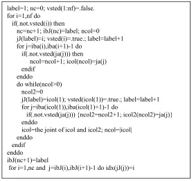
[image:4.612.149.461.140.492.2]In the aggregation schemes based on strong connections, Braess scheme or Vanek scheme, strongly coupling is the core concept. The process to match between grid-points is often based on this concept, but in general only two points are matched each time. May we select several points each time and how to select?
Figure 2. The Braess aggregation algorithm.
In this section, an aggregation algorithm based on clique is given. In this algorithm, a non-visited point i is found each time and all the non-visited adjacent points are recorded in set icol. Then a point from icol is picked up and its non-visited adjacent points are recorded in icol2. Finally, the joint of icol and icol2 is computed and assigned to icol to start a new loop. In this way, finally a maximum clique containing i can be found and it is put into jJ. The algorithm is denoting as aggcq and the details can be referred to figure 4.
Numerical Experiments
In this paper, all experiments are done on a processor of Intel(R) Xeon(R) CPU E5-2670 [email protected] (cache 20480 KB). The operating system is Red Hat Linux 2.6.32-279- aftms-TH and the compiler is Intel FORTRAN Version 11.1.
For the derived linear systems are all symmetric positive definite, PCG is used all the time. The initial iteration vector is selected as the zero and the iteration is stopped when the ratio of the Euclid norm of the current residual vector to that of the initial one is
vsted(1:nf)=.false.; label=1; nk=0 for it=1,nf do
if(.not.vsted(it)) then
nk=nk+1; ibK(nk)=label; jK(label)=it; label=label+1 find the non-visited adjacent points of it and put into set Z find the point jt with strongest connection from Z if(jt exist) {jK(label)=jt; vsted(jt)=.true.; label=label+1} endif
enddo
ibK(nk+1)=label; vsted(1:nf)=.false.; label=1; nc=0 for it=1,nk and jx=ibK(it),ibK(it+1)-1 do idx(jK(jx))=it for it=1,nk do
if(.not.vsted(jK(ibK(it)))) then nc=nc+1; ibJ(nc)=label for jx=ibK(it),ibK(it+1)-1 do
jJ(label)=jK(jx); vsted(jK(jx))=.true.; label=label+1 enddo
denote jK(ibK(it):ibK(it+1)-1) as U for jt in [1,nk] and not equals to it, do denote jK(ibK(jt):ibK(jt+1)-1) as V
set nnz(k) to the number of connection between U and V enddo
find jmax such that nnz(jmax) is the maximum in nnz for jx=ibK(jmax),ibK(jmax+1)-1 do
jJ(label)=jK(jx); vsted(jK(jx))=.true.; label=label+1 enddo
endif enddo
ibJ(nc+1)=label
smaller than 1E-10 or the maximum number of iterations 3000 is attained. For multigrid methods, the coarsening process is stopped when the number of points is less than 100. The linear system on the coarsest level is solved with ILU (0) PCG iteration and the stop criterion is 1E-10 too.
Figure 3. The Vanek aggregation algorithm
The computation time is dependent on the non-zero entries of the coefficient matrix on each level, and the number of iterations. Thus, these parameters are counted in all experiments. In all the tables, Nlev denotes the number of levels of the multigrid, Cgrd denote the complexity of the grids, that is, the ratio of the total number of grid points on each level to that on the finest level. Cop denotes the complexity of the operators, that is, the ratio of the total number of non-zeros in the coefficient matrices on each level to that on the finest level. ItsJA and itsGS denote the number of iterations required when Jacobi or Gauss-Seidel is selected as the smoother respectively, itmJA and itmGS denote the related time used in seconds for iteration. In addition, sttm denotes the time
label=1 for it=1,nf do ibN(it)=label
for each jt strongly coupled to it, do jN(label)=jt; label=label+1 enddo
enddo
ibN(nf+1)=label; nJ=0; label=1
put those non-isolated points to U and copy U to V do while |U|>0
i=U(1)
if(jN(ibN(i):ibN(i+1)-1) is in V) then nJ=nJ+1; ibJ(nJ)=label
for j=ibN(i),ibN(i+1)-1 do {jJ(label)=jN(j); label=label+1} U=U\jN(ibN(i):ibN(i+1)-1); V=V\jN(ibN(i):ibN(i+1)-1) else
U=U\{i} endif enddo
ibJ(nJ+1)=label; nJt=nJ; ibJt=ibJ; jJt=jJ
record the element for each of the nJ sets with linked list copy V to U
do while(|V|>0) i=V(1); V=V\{i} for k=1,nJ do
S=the joint of jN(ibN(i):ibN(i+1)-1) and jJt(ibJt(k):ibJt(k+1)-1) if(|S|>0) {add i to the k-th linked list; U=U\{i}}
enddo enddo
recover ibJ and jJ from the new linked list do while(|U|>0)
i=U(1); nJ=nJ+1; ibJ(nJ)=label
S=the joint of jN(ibN(i):ibN(i+1)-1) and U for j=1,nS do {jJ(label)=S(j); label=label+1} U=U\S
enddo
ibJ(nc+1)=label
used in seconds for set-up, and ttmJA and ttmGS denote the related total time including the setup time and the time for iteration.
Figure 4. The aggregation algorithm based on clique
Experiments are performed for four linear systems, namely LinSys21, LinSys22, LinSys31 and LinSys32. All these linear systems are derived with finite difference method. The former two are derived from 2D PDE problem with Dirichlet boundaries
. 2 2 2 2 f y u x u = ∂ ∂ − ∂ ∂
− (2)
The definition region is (0,1)×(0,1) and the function f and the boundary values are given from a known true solution u=1. There are n+2 points spaced evenly in each dimension and the value u(xi,yj) is defined as ui,j for any continuous function u. For linear system LinSys21, the following discrete form is used
. 4 1, , 1
, 1 1
,j i j ij i j ij ij
i u u u u f
u − + − − =
− − − + + (3)
For linear systems LinSys22, the discrete form used is
. 4
4 20 4
4 , 1 1, 1 1, , 1, 1, 1 , 1 1, 1
1 ,
1j ij i j i j ij i j i j ij i j ij
i u u u u u u u u f
u − − − + − − − − =
− − − − + − − + − + + + + (4)
LinSys31 and LinSys32 is from a 3D PDE problem with Dirichlet boundaries
. 2 2 2 2 2 2 f z u y u x u = ∂ ∂ − ∂ ∂ − ∂ ∂
− (5)
The definition region is (0,1)×(0,1)×(0,1) and f and the boundary values are given from a known true solution u=1. There are n+2 points spaced evenly in each dimension and u(xi,yj,zk) is denoted as ui,j,k for any function u. For linear system LinSys31, the following discrete form is used
label=1; nc=0; vsted(1:nf)=.false. for i=1,nf do
if(.not.vsted(i)) then
nc=nc+1; ibJ(nc)=label; ncol=0
jJ(label)=i; vsted(i)=.true.; label=label+1 for j=iba(i),iba(i+1)-1 do
if(.not.vsted(ja(j))) then ncol=ncol+1; icol(ncol)=ja(j) endif enddo do while(ncol>0) ncol2=0
jJ(label)=icol(1); vsted(icol(1))=.true.; label=label+1 for j=iba(icol(1)),iba(icol(1)+1)-1 do
if(.not.vsted(ja(j))) {ncol2=ncol2+1; icol2(ncol2)=ja(j)} enddo
icol=the joint of icol and icol2; ncol=|icol| enddo
endif enddo
ibJ(nc+1)=label
. 6 ,, 1,, , 1, ,, 1 , , 1 , 1 , 1 ,
,jk i j k i jk i jk i jk i j k ijk ij
i u u u u u u f
u − − + − + + =
− − − − + + + (6)
For linear systems LinSys32, the discrete form used is
. 27 ,, 1 1 ' 1 1 ' 1 1 ' ' ,'
,' ijk ij i i i j j j k k k k j
i u f
u + =
−
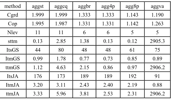
+ − = + − = + − = (7)The experiment results are given in table 1 to table 4. It is clear that, for aggva, the number of levels is always the smallest and the setup or the total computation time is always the largest.
[image:7.612.160.455.289.460.2]We can see from table 1 that, with agg8p, the complexity of the grid and operator, and the number of levels are all the smallest. And with scheme aggva, the complexity parameters are all the second. When Jacobi is used as smoother, as for the performance of iteration, aggva is the best. But when Gauss-Seidel iteration is used as smoother, agg8p is the best, and agg4p is the second. As for the total time used, agg8p is the best for Jacobi smoothing, and agg4p is the best for Gauss-Seidel smoothing.
Table 1. Results from PCG with n=256 for LinSys21.
method aggst aggcq aggbr agg4p agg8p aggva
Cgrd 1.999 1.999 1.333 1.333 1.143 1.190
Cop 1.995 1.987 1.331 1.331 1.142 1.263
Nlev 11 11 6 6 5 5
sttm 0.13 2.85 1.38 0.13 0.12 2905.3
ItsGS 44 80 48 48 61 75
ItmGS 0.99 1.78 0.77 0.73 0.85 0.89
ttmGS 1.12 4.63 2.15 0.86 0.97 2906.2
ItsJA 176 173 189 189 192 91
ItmJA 3.20 3.11 2.43 2.40 2.19 0.88
ttmJA 3.33 5.96 3.81 2.53 2.31 2906.2
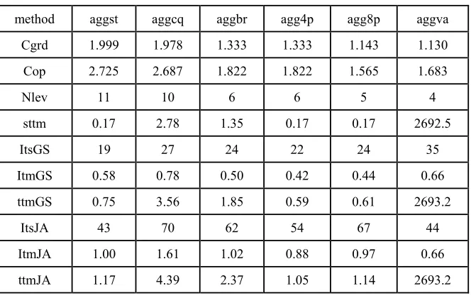
We can see from table 2 that, for LinSys22, as for the complexity, aggva is the best and agg8p has similar performance. As for the setup time, agg8p is the best, and agg4p and aggst both have similar results. As for the performance of iteration, aggva is always the best for either of the two smoothers.
Table 2. Results from PCG with n=256 for LinSys22.
method aggst aggcq aggbr agg4p agg8p aggva
Cgrd 1.999 1.333 1.333 1.333 1.143 1.127
Cop 3.578 2.389 2.389 2.389 2.049 2.021
Nlev 11 6 6 6 5 4
sttm 0.22 3.40 1.84 0.21 0.20 13.45
ItsGS 43 47 47 47 60 48
ItmGS 1.51 1.11 1.11 1.17 1.24 0.80
ttmGS 1.73 4.51 2.95 1.38 1.44 14.25
ItsJA 44 47 47 47 63 53
ItmJA 1.31 0.96 0.96 0.94 1.13 0.75
ttmJA 1.53 4.36 2.80 1.15 1.33 14.20
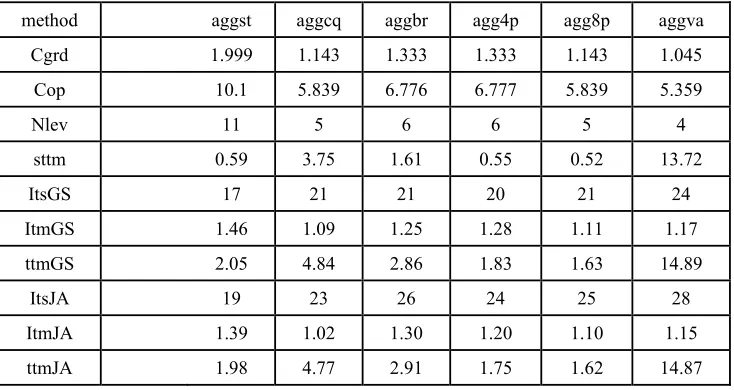
It can be seen from table 4 that, for LinSys32, as for the complexity, aggva is the best. As for the setup time, agg8p is the best. As for the performance of iteration, when Jacobi smoothing is used, aggcq is the best. When Gauss-Seidel smoothing is used, aggcq is the best, but both agg8p and aggva can achieve similar results.
In addition, from table 1 to table 4, the more complex the coefficient matrix of the initial linear system is, relatively the less setup time and the more efficient the scheme aggva will be. The more points each point connects to in average, the more efficient the scheme aggcq will be. And agg8p needs always the least setup time. Though aggst, agg4p and agg8p are all very cheap to setup, the performance of iteration is also very good, and the best is often one of them in most cases. Even if they are not the best, the performance is not far from the best. It should be mentioned that though there give only the results from three test examples, many other tests give the similar results.
Table 3. Results from PCG with n=40 for LinSys31.
method aggst aggcq aggbr agg4p agg8p aggva
Cgrd 1.999 1.978 1.333 1.333 1.143 1.130
Cop 2.725 2.687 1.822 1.822 1.565 1.683
Nlev 11 10 6 6 5 4
sttm 0.17 2.78 1.35 0.17 0.17 2692.5
ItsGS 19 27 24 22 24 35
ItmGS 0.58 0.78 0.50 0.42 0.44 0.66
ttmGS 0.75 3.56 1.85 0.59 0.61 2693.2
ItsJA 43 70 62 54 67 44
ItmJA 1.00 1.61 1.02 0.88 0.97 0.66
[image:8.612.142.474.476.686.2]Table 4. Results from PCG with n=40 for LinSys32.
method aggst aggcq aggbr agg4p agg8p aggva
Cgrd 1.999 1.143 1.333 1.333 1.143 1.045
Cop 10.1 5.839 6.776 6.777 5.839 5.359
Nlev 11 5 6 6 5 4
sttm 0.59 3.75 1.61 0.55 0.52 13.72
ItsGS 17 21 21 20 21 24
ItmGS 1.46 1.09 1.25 1.28 1.11 1.17
ttmGS 2.05 4.84 2.86 1.83 1.63 14.89
ItsJA 19 23 26 24 25 28
ItmJA 1.39 1.02 1.30 1.20 1.10 1.15
ttmJA 1.98 4.77 2.91 1.75 1.62 14.87
Conclusions
In this paper, a new method based on cliques and several classical aggregations are implemented based on sparse data structures, and compared in solving sparse linear systems from model partial differential equations. The results show that Vanek algorithm has the least number of levels all the time, and as for performance of iteration, when Jacobi is used as the smoother, it is also the best in general. When Gauss-Seidel smoother is used, it is the best in many cases too. But the setup time is always very long, which makes it have no privileges to any others in respect of total computation time. The two-point aggregations based on strong connections, and their modification versions based on loop two or three times are effective too. In most cases, the best scheme is one of these three algorithms. Even if they are not the best, the results are not far from the best. And the more points of each point connect to in average, relatively the less time the Vanek scheme require to setup and relatively the more efficient it is, so is the aggregation algorithm based on cliques.
Acknowledgement
This research was financially supported by NSFC (61379022).
References
[1] J. W. Ruge and K. Stuben. Algebraic multigrid, Multigrid Methods. In: Frontiers of Applied Mathematics, vol.3. SIAM Philadelphia, PA. 1987, pp.73-130.
[2] R. Wienands, W. Joppich. Practical Fourier analysis for multigrid methods, Taylor and Francis Inc. 2004.
[3] K. Stuben. A review of algebraic multigrid. J. Comput. Appl. Math. and Applied Mathematics. 128(2001) 281-309.
[5] H. Kim, J. Xu, and L. Zikatanov. A multigrid method based on graph matching for convection-diffusion equations. Numer. Linear Algebra Appl. 10(2003)181–195. [6] P. D'Ambra, A. Buttari, D. di Serafino, S. Filippone, S. Gentile, B. Ucar. A novel aggregation method based on graph matching for algebraic multigrid preconditioning of sparse linear systems, in: International Conference on Preconditioning Techniques for Scientific & Industrial Applications. 2011, May 2011, Bordeaux, France.
[7] D. Braess. Towards algebraic multigrid for elliptic problems of second order, Computing. 55(1995)379-393.
[8] P. Vanek, J. Mandel, and M. Brezina. Algebraic multigrid by smoothed aggregation for second order and fourth order elliptic problems. Computing. 56(1996)179-196.