KEVIN SCULLY
Received 1 September 2004 and in revised form 20 December 2004
This paper presents a globalL1-estimate for the convergence of mesh-based interpolants
on 2-manifolds defined over multiple coordinate systems and analyzes the convergence of an integral on a triangulated approximate manifold to the desired integral on the man-ifold being approximated. To place this estimate in context, previous convergence esti-mates for interpolation techniques on manifolds are presented. Finally, numerical results demonstrating the value of theL1-estimate are presented.
1. Introduction
Mesh-based interpolation (e.g., finite-element interpolation) of functions defined on sur-faces and manifolds has received attention in a diverse range of applications including computer graphics [3], structural engineering [5], and astrophysics [11]. In many of these applications, the domain in question possesses substantial curvature or discontinuities in its tangent plane and can only be described nonsingularly with multiple coordinate sys-tems. In these scenarios, subtle details of approximation, unseen in the traditional frame-work, arise which may prevent convergence [2,14].
To elucidate these details, this paper presents a global L1-convergence estimate for
mesh-based element interpolants on 2-surfaces (and 2-manifolds). To place this estimate in context, we offer a brief survey of efforts to construct interpolants on manifolds for Petrov-Galerkin methods. (A more thorough survey appears in [18].)
This survey will examine Nedelec’s approach as described in [17] which has served as a standard for finite-element approximation across multiple coordinate systems. This survey will also discuss techniques not requiring a traditional mesh. These “meshless” methods provide context in two ways. First, they illustrate the use of globalLp-estimates,
1≤p <∞, on manifolds. We will place mesh-based methods into a comparable frame-work, in contrast to theL∞- and localLp-estimates traditionally used. Second, meshless
methods which decompose a subset ofRninto a covering of open sets parallel the use of
open coverings in a manifold representation.
Before reading the survey, note the following technical point. The majority of the methods on manifolds surveyed have been developed for 2-surfaces lying inR3, which
up to equivalence, do not encompass all 2-manifolds. For example, Nedelec, Sheng, and
Copyright©2005 Hindawi Publishing Corporation
Hirsch specifically exploit the structure of a 2-surface inR3to build their framework. The
central result of this paper, by contrast, is built only from the manifold structure of the 2-manifold and applies more generally. However, to address the motivating examples for this result, this paper focuses mainly on 2-surfaces lying inR3.
1.1. Mesh-based approaches. The challenge in developing mesh-based approaches to approximation on manifolds lies in relating the viewpoints of classical differential ge-ometry and numerical approximation. In classical differential geometry, the different coordinate systems (also called “patches” or “charts”) are blended together via smooth “partition-of-unity” functions, which then permit the definition of globally defined quan-tities (e.g., integrals) via the patches. The smoothness of the partition functions require substantial overlap among their supports and these support sets will frequently not be polygonal. Mesh-based interpolation, by definition, however, requires a polygonal de-composition of the underlying set. Also, in practice, numerical methods on manifolds favor disjoint partitions of manifolds [1,14] which correspond to piecewise constant, discontinuous partition-of-unity functions, and thus, lie outside the framework of clas-sical, differential geometry.
One sees these assumptions of no overlap among the charts and polygonal chart sets in the work of Nedelec. Further, we see the use of globalL∞-estimates, in Nedelec’s work and the work of Sheng and Hirsch, thereby circumventing the difficulties in defining global integration when the classical differential geometric framework does not apply.
1.1.1. Nedelec’s work. Nedelec [17] delivered some of the first surface approximation er-ror estimates. He begins with ppatches, polygonal sets{Si}which, together with maps
Φi, form the surface. The sets{Si}partition the manifold disjointly, that is, they intersect
only at their boundaries. He triangulates eachSiand constructs on each triangleT ofSi
an interpolantFT from a space containing all polynomials up to degreek of the chart
functionΦi. He then stitches eachFT together to form aC0-functionΦihonSiwhich is
locally differentiable on eachT. For the greatest diameterhacross each triangulation of eachSi, the following estimates hold:
max
i=1···psupx∈Si
Φi(x)−Φih(x)≤Chk+1 max i=1···psupx∈Si
Dk+1Φ i(x),
max
i=1···p supx∈Si
DlΦ
i(x)−DlΦih(x)≤Chk+1−l max i=1···psupx∈Si
Dk+1Φ
i(x)1≤l≤k+ 1,
(1.1)
where| · |refers to the standard vector or matrix norm. Nedelec then asserts, for suffi-ciently smallh, the existence of a homeomorphismψbetween this approximate surface and the original surface whose inverse associates to each pointpon the original surface the point on the approximate surface intersecting the surface normal atp. Viaψ, the tri-angulation of the approximate surface becomes a tritri-angulation of the original surface. He then proves that, forFTand the functionψ·FTfromSito the original surface,
sup
x∈T
ψ·FT(x)−FT(x)≤Chk+1sup x∈T
Dk+1Φ i(x)
sup
x∈T
D
ψ·FT(x)
−DFT(x)≤Chksup x∈T
Dk+1Φ i(x).
He then gives estimates for the determinantsJ(·) of the metrics formed by these chart functions:
sup
x∈T
J
Φi(x)−JFT(x)≤Chksup x∈T
Dk+1Φ
i(x), (1.3)
sup
x∈T
J
ψ·FT(x)−JFT(x)≤Chk+1sup x∈T
Dk+1Φ
i(x). (1.4)
Note that the existence of ψ increases the expected order of convergence from the standard interpolation framework. In the forthcoming [19], we will demonstrate that this faster estimate holds whenD2Φ
i∞is finite and the surface is tangent plane continuous.
1.1.2. Sheng and Hirsch. The engineering-inspired field of “parametric surface meshing” is devoted to mesh-based interpolation of functions on surfaces. The following theorem of Sheng and Hirsch (see [20]) represents one of the most often cited convergence theo-rems in this field and again, employs anL∞-estimate.
Theorem1.1. LetS(u,v)be aC2-smooth parametric patch defined on[a,b]×[c,d]. Let
T∈[a,b]×[c,d]be an arbitrary triangle with vertices(A1,A2,A3)in the parametric space,
and lethbe the maximal edge length of the triangle. Then, linear interpolantST ofSsuch thatST(Ai)=S(Ai)satisfies
sup
(u,v)∈T
S(u,v)−ST(u,v)≤2 9h
2M
1+ 2M2+M3, (1.5)
where · is the Euclidean R3-norm and M
1 = sup(u,v)∈T∂2S(u,v)/∂u2, M2 =
sup(u,v)∈T∂2S(u,v)/∂u∂vandM
3=sup(u,v)∈T∂2S(u,v)/∂v2.
1.2. Non-mesh-based approaches. The preceding mesh-based approaches use L∞
-estimates and rest on classicalCk-differentiability. We will see that the chart functions
and the related transition functions are better described by weak differentiability and Sobolev spaces, that is,Wk,p, the space of functions with weak derivatives up to orderk
lying inLp. The following non-mesh-based estimates provide a framework more natural
for weak differentiability and on a related note, globalLp-estimates, 1≤p <∞. The first
set of estimates use an alternative formulation of weak differentiability via Fourier series. 1.2.1. Interpolation on manifolds via Fourier series. The interpolation of anL2(=W0,2
)-orHk(=Wk,2)-function on a manifold, given a sampling of its values (either measured
under an integral sign or measured pointwise after making assumptions to clarify the almost everywhere ambiguity ofL2-functions), via the construction of interpolants based
on Fourier series has been studied in the papers [8,9,16]. Often the interpolants are built from “radial basis functions” which vary only according to the radial distance from a fixed point [16]. With these Fourier series representations, the original functions and their interpolants are analyzed in terms of Sobolev spaces built from examining the decay of coefficients in the functions’ Fourier series. Many approximation results on spheres and tori have been developed in this framework.
a finite number of terms. Then, they approximate the truncated series with an interpolant IΦ,X(fL) built from a kernelΦand a discrete subsetXof the original domainΩ. From this
setX, we may derive a “mesh norm”h:=maxy∈Ωminx∈Xd(x,y). This norm measures,
through the metricd(x,y) ofΩ, the furthest distance a point inΩmay lie from a point inX. Under the assumption that card(X)=O(h−n), wherenis the dimension ofΩand
card(X) refers to the number of elements inX, they prove an estimate of the form
f −IΦ,X
fL∞,Ω=O
hσ−n/2f
w, (1.6)
whereσ measures the rate of decay of the coefficients of f and thew-norm measures these coefficients relative to certain “weights.”
1.2.2. Meshless methods. Non-mesh-based interpolation techniques, such as those de-scribed above, have given rise to “meshless methods.” These Petrov-Galerkin methods for discretizing systems of partial differential equations without a mesh seek to elim-inate the burdensome storage and time requirements of managing a mesh. The chal-lenge these methods face lies mainly in numerical integration. The bottleneck in using Petrov-Galerkin methods to solve PDEs lies in solving the large matrices produced by discretizations of the integrated “weak form” equations. To make computations feasible, these matrices must be sparse. To create sparse matrices, the functions used must have local support and the construction of local support requires a decomposition of the do-main into smaller pieces. Thus, while many of these meshless methods do not use meshes for interpolation, they use meshes for integration. Other methods do not use polygonal meshes, but use structures comparable to meshes, such as a spherical decomposition of the domain to define integration. In general, meshless methods have been found to be less efficient than mesh-based methods [4]. In fact, the architects of one such method later incorporated the polygonal meshes into their previous framework to avoid the difficulties caused by the lack of such a mesh [6,7].
Among the meshless methods, two methods, in particular, lay theoretical groundwork for finite-element (and more generally, mesh-based) methods on manifolds. Both the partition-of-unity method [15] and the hp-cloud method [6] construct interpolants from partitions of unity built from an open cover of the domain. The parallels between open covers of sets inRnand open covers of manifolds make these two methods relevant to
this discussion. In each method, a function is approximated locally and from these lo-cal approximations, a global approximation is produced via the partition of unity. The key difference between these methods lies in the number of open sets in the covering. The partition-of-unity method more closely relates to our work, but the similarity and simultaneous arrival of the hp-cloud method make this method worthy of our attention. In the partition-of-unity method, there is not necessarily an a priori relationship be-tween the number of “patches” (open sets) and the rate of the convergence or bebe-tween the size of the patches and the rate of convergence. While such relationships may exist in implementations of this method, the underlying theory only assumes the existence of 1(i) and2(i) which bound the approximations on each patch. These’s alone control
the rate of convergence in the first global estimate below. In the second estimate,1(i)
This requirement, however, does not impose a functional relationship between the two. Thus, the number of patches may be ofO(1) if the convergence of these(i)’s to zero does not depend on the number of patches or the area of these patches. Here, we offer the central results underlying this method.
Theorem1.2 (Melenk and Babuska). LetΩ⊂Rn. Let{Ω
i}be an open cover ofΩsuch that each point inΩlies in only at mostMof theΩi. Let{φi}be a partition-of-unity subordinate to this cover such that there exist constantsC∞andCGsuch that
φi
L∞(Rn)≤C∞, ∇φiL∞(Rn)≤
CG
diamΩi. (1.7)
LetVi⊂H1(Ωi∩Ω)andV=
iφiVi. Letu∈H1(Ω). Suppose that for eachi, there exists
vi∈Vi,1(i)and2(i)such that
u−vi
L2(Ω
i∩Ω)≤1(i),
∇
u−viL2(Ω
i∩Ω)≤2(i). (1.8)
Then, the functionuap=
iφivi∈V⊂H1(Ω)satisfies
u−uap
L2(Ω)≤
√ MC∞
i 2
1(i)
1/2
∇
u−uapL2(Ω)≤
√ 2M
i
CG
diamΩi
2
2
1(i) +C2∞22(i)
1/2
.
(1.9)
Thus, we expect the order of the global approximation to be that of the local approxi-mation.
In contrast to the partition-of-unity method, the hp-cloud method explicitly creates the local approximation space and bounds the error in this local approximation space as a function of the size of the open sets. The hp-cloud method decomposes the do-main intoO(h−n) open ballsωh
α, with each set occupying an area ofO(hn), wherehis
the maximum of the dilation parameters hα of the affine maps which send the open
balls to the unit ball. The local approximation spaces are constructed from the parti-tion funcparti-tions whose supports intersect the given patch and from the product of these partition functions with polynomials. An estimate measuring the difference between a functionu∈Wp+1(Ω∩ωh
α) and its local interpolantΠ2αuis proven under comparable
assumptions to those of the partition-of-unity method: each partition function satisfies φh
αL∞(Ω)≤C∞and∇φhαL∞(Ω)≤CG/hαand each point ofΩis contained in at mostM
charts. A simplified version of this estimate follows:
u−Π2
αum,2,Ω∩ωh α≤Cαh
p+1−m
α |u|p+1,2,Ω∩ωh
α, (1.10)
those of the partition-of-unity method:
u−uhp
L2(Ω)≤MC∞max α Cαh
p+1u Hp+1(Ω),
u−uhp
H1(Ω)≤
√ 2Mmax
α
CGCα+C∞Cα
hpu
Hp+1(Ω).
(1.11)
Both these methods invoke a partition of unity to combine local approximations into a global approximation and their approaches provide insight into mesh-based approxi-mations on manifolds. Recall, however, that classical partitions of unity often do not give rise to polygonal decompositions of the manifold. In such a case, an approximate parti-tion of unity and an approximate polygonal decomposiparti-tion of the manifold will be used. The question then arises of how well the triangulation approximates the manifold.
2. Comparing functions on different manifolds
2.1. Defining a metric. To measure the error in a mesh-based approximation of a func-tion on a manifold, we must somehow evaluate the difference between the triangulated manifold and the manifold it approximates. We will call two manifoldsMandN equal if there exist a cover ofM,{Ci},Ci⊂Rn, and a cover ofN,{Di},Di⊂Rn, and maps
γM,i:Ci →MandγN,i:Di →Nsuch that for alli,Ci=Dia.e. andγM,i−γN,iWk,p(Ci)=0.
(The choice ofp=2 seems the most natural for a framework for solving PDEs, butp=1 appears to be the most theoretical satisfying choice, per our discussion below.)
This notion of equivalence of manifolds suggests a way of judging when two manifolds are “close.”MandNare approximately equal if they have comparable charts structuresCi
andDi, respectively, whose symmetric differenceCi∆Diis small, and associated mapsγM,i
andγN,iwhich are both well-defined and nonsingular onCi∪Di, and whose difference
is small in aWk,p-norm. With this viewpoint for evaluating the difference between two
manifolds, we may define a “metric” (topologically speaking, a pseudometric) for eval-uating the difference between two functions onMandN. The crucial idea is that while γM,ineeds only to be defined onCifor purposes of constructingM, its definition may be
extended to areas ofDinot inCiwithout difficulty. We propose to measure the difference
between a function f onMand a functionqonNvia the following function:
dM,N(f,q)=
i
φM,if
gM−φN,iqgNL1(C
i∪Di). (2.1)
(By an abuse of notation, we refer to f both as a function fromM →Rand via a chart map as a function fromCi →R.) Here,φM,iandφN,irefer to partitions of unity on their
respective manifolds andgMandgNare the determinants of the metrics of their respective
manifolds. Observe thatdM,M(f,q)= f−qL1(M). (We assume that the same charts and
partition of unity are used in both treatments ofM.) Further,
Mf −
Mh
f≤dM,Mh
f,fh
We now have a means for measuring our approximation of a function f on a manifold. We will demonstrate that this approximation depends upon our ability to approximate the functionf on each chart, our ability to approximate the partition of unity functions, and our ability to approximate the determinant of the metric which derives from our abil-ity to approximate the manifold. This observation is the essence ofLemma 2.1to follow. TheL1-norm, as opposed to anotherLp-norm, appears in the definition for several
reasons. First, because transition functions and chart maps will not take infinite values, the derivatives of transition functions and chart maps should have finiteL1-norm. This
claim will not necessarily hold true for theLp-norm, p >1. Also,d
M,N reduces to the
L1-norm onM whenM=Nand the use of theL1-norm appears to offer better
conver-gence compared to alternatives we have considered. If we replaceL1withL2,d
M,Nwill not
reproduce theL2-norm whenM=N. Additionally, with this definition, using the
tech-niques of the proof ofLemma 2.1below, theL1-norm appears to give a better convergence
estimate (although this difference may just be a product of number manipulation in our efforts to find the most appropriate measurement). We could also replace theL1-norm
withL2-norm and take the square roots of the partition functions and the fourth roots
of the metric determinants. While this choice reproduces theL2(M)-norm whenM=N,
it appears to give a lower order estimate in the approximation of the partition functions. Finally, note that since the sets in question are of finite measure, we may bound theL1
-norms by multiples of theL2-norms:
fL1≤ fL2
mA. (2.3)
2.2. Local (one-chart) error estimates. In the following lemma, we will take a chartC of a 2-manifoldMand approximate it with a triangulationD, one part of a global trian-gulated approximationMh. We will then bound the individual terms in the sum indM,Mh
in terms of the approximations of its component parts: the function f, the partition of unity function, and the square root of the metric determinant. These errors are taken over D, assuming that these functions are defined on areas ofDoutside ofC. Extending these errors over all ofD, instead of over all triangles inDcompletely contained inC, appears to give rise to better higher-order approximation.
In the following lemma, we place no explicit restrictions on the differentiability ofM. We place implicit restrictions onMby assuming the metric determinant is inL∞. Fur-ther, we implicitly restrict the differentiability ofM by assuming that the chart sets have piecewiseWr,1boundaries since these boundaries are defined by transition functions. We
may assume that the chart maps ofMlie inWk1,p,k
1>1, and the transition functions lie
inWk2,p,k
2≥1. We will see that the differentiability of these functions will influence the
rates of convergence of the different terms in the following estimate.
Lemma2.1. LetC⊂R2be a single chart set, a bounded, connected set with a piecewiseWr,1
boundary,r=1or2, of a2-manifoldM. LetCbe approximated by a triangulated polygon D such that each boundary edge ofD is the linear interpolant of aWr,1-segment of the
boundary curve ofC. Thus, there exists a set of intervals[aj,bj]partitioning the boundary ofCinto curve segments such that on each segment, the boundary ofCis given byw=zj(u),
z∈Wr,1([a
CandD are contained in larger charts so that areas ofD not inCare defined and that the Lebesque measurem(C∪D)is finite. Lethbe the maximum of the edge lengths of the triangles inD. Letf be a function defined onM,φa partition of unity function for a covering ofM containingC, andg the determinant of the metric components. Let fh,φh, andgh be the respective approximations of f,φ, andgdefined onDand0outsideD. Assume that all functions and their respective approximations are bounded above, both inL1andL∞-norms onC∪D. Suppose there exists>0which bounds|g|and|gh|from below, that is, that both metrics are nonsingular. Assume that the number of boundary triangles is at mostO(1/h). Then, there exists a constantKsuch that the following estimates hold:
φ f|g| −φhfh
|gh|L1(C∪D)
≤Kφ−φhL1(D)+f−fhL1(D)+|g| −ghL1(D)+hr
.
(2.4)
Proof.
φ f|g| −φhfh
|gh|L1(C∪D)
=φ−φh
f|g|+f−fh
φh
|g|+|g| −ghφhfhL1(C∪D)
≤φ−φhf
|g|
L1(C∪D)+
f −fhφh
|g|
L1(C∪D)
+|g| −ghφhfhL1(C∪D)
≤φ−φhL1(C∪D)fL∞(C∪D)
|g|
L∞(C∪D)
+f −fhL1(C∪D)φhL∞(C∪D)
ghL∞(C∪D)
+|g| −ghL1(C∪D)φhL∞(C∪D)fhL∞(C∪D).
(2.5)
Now, for the sake of simplicity, we will replace theseL∞-norms with a constantK:
φ f|g| −φhfh
|gh|L1(C∪D)
≤K φ−φhL1(C∪D)+f −fhL1(C∪D)+
|g| −ghL1(C∪D)
≤K φ−φhL1(C−D)+f −fhL1(C−D)+
|g| −ghL1(C−D)
+φ−φhL1(D)+f −fhL1(D)+
|g| −ghL1(D)
.
And since all of the functions in question are bounded from above in L∞(C∪D), the preceding quantity is
φ f|g| −φhfh
|gh|L1(C∪D)
≤K 1L1(C−D)+φ−φh
L1(D)+f−fhL1(D)+
|g| −ghL1(D)
(2.7)
(1 is the unit constant function)
K 1L1(C−D)+φ−φhL1(D)+f −fhL1(D)+
|g| −ghL1(D)
=K m(C−D) +φ−φhL1(D)+f−fhL1(D)+
|g| −gh L1(D)
.
(2.8)
C−Dconsists of regions formed where the boundary curves ofCwander outside the triangles. Since we have assumed each edge ofDis the piecewise linear interpolant of a boundary curve, we have
m(C−D)≤
j
[aj,bj]
dj(v)−πh
dj(v)dv. (2.9)
Here πh(dj) is the linear interpolant of dj, that is, dj(aj)=πhdj(aj) and dj(bj)=
πhdj(bj). (Note that the above sum also includes D−C.) Also, (v,u)=(x,y) or (y,x)
where (x,y) is the coordinate system ofCi, that is,uandvvary from triangle to triangle
depending on whether it makes more sense to describe yas function ofxor vice versa. From interpolation theory, we have
[aj,bj]
dj(v)−πh dj
(v)dv≤Khr
[aj,bj]
d(r)
j dv, (2.10)
and since|d(jr)|is bounded in integral,
m(C−D)≤
j
Khrb j−aj
≤
j
Khr+1, (2.11)
and since the number ofjisO(1/h),
m(C−D)≤Khr. (2.12)
We now turn to the approximation of the square roots of the metric determinants. Observe
|g| −gh=
|g| −gh
|g|+gh
≤ 1 2√
|g| −gh. (2.13)
Corollary2.2. Suppose thatCis polygonal, that is, thatCmay be triangulated exactly and D=C. ThenC∪D=D=Cand thehrterm may be removed from the preceding estimate. (In this case, we will most likely use the same partition function and the term involving partition functions may also be removed.)
2.3. Global estimates. By summing the local estimates, chart by chart, into a global re-sult, we obtain the following theorem.
Theorem2.3. LetMbe a 2 manifold covered by charts{Ci}, with piecewiseWr,1,r=1or
2, boundary curves, with associated partition of unity functions{φi}. (This may be an almost everywhere partition; that is, the partition of unity equations may fail on a set of measure 0.) For eachi, letDibe a triangulation ofCisuch that each boundary edge ofDiis the linear interpolant of aWr,1boundary curve ofC
i. Assume that the chart maps toMfromCihave a well-defined, one-to-one extension toCi∪Di. LetMh refer to the manifold defined by{Di} and the approximate chart maps. Letf be a function onMandgthe metric. Letφh,i,fh, and
ghbe local approximations toφi, f, andg, respectively. Assume that the metric determinants are bounded away from zero. (We will also use fhto refer to the function onMhwhich locally equals fh.) Lethbe a parameter which bounds from above, within a constant, the lengths of the sides of the triangles in eachDi. LetJrefer to the number ofCifor whichm(Ci−Di)>0. Then, the following estimate holds:
dM,Mh
f,fh
≤K
i
φi−φh,iL1(D
i)+
f −fh
L1(D
i)+
|g| −gh
L1(D
i)
+Jhr
.
(2.14)
Thus, to understand the rate of convergence of an approximate integral, we must ana-lyze the rate of convergence of each term in the estimate. For each respective term, we ask ourselves the following questions.
(1) What is the partition of unity? In the absence of an exact partition of the chart into triangles, the convergence of the partition of unity term is generally given by the smoothness of the transition functions.
(2) What interpolation scheme approximates f?
(3) Does the faster convergence of the inequality (1.4) apply? More specifically, does the surface haveL∞-bounded second derivatives of the chart to surface maps and a continuous tangent plane? If not, what is the differentiability of the chart maps? (A generalization of (1.4) to weakly differentiable chart maps appears in [19].) (4) What is the differentiability of the boundary of each chart, that is, what isr?
Like the convergence of the partition of unity term, this question depends on the smoothness of transition functions.
This estimate provides a framework by which we may evaluate approaches for approx-imating functions on manifolds. The work [18] examines several of these approaches in light of this framework, clarifying the limitations and underlying assumptions of such techniques. These approaches include the expression of a 2-dimensional, polygonal mesh inR3as a manifold by constructing charts out of all polygons containing a given vertex
1.4 1.2 1 0.8 0.6 0.4 0.2 0 2
1.5 1
0.5
0 0 0.5
[image:11.468.141.325.69.207.2]1 1.5 2
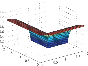
Figure 3.1. Two cylindrical patches.
Most approaches for triangulating a covering of a manifold will ignore the issue of overlap and gaps formed when triangulating each chart and treat the boundaries of each chart triangulation as if they align exactly. The partition of unity functions is gener-ally ignored in such implementations, and by default, are taken to be the characteris-tic functions of their corresponding charts (i.e., a disjoint partition is used). The term φi−φi,his then bounded by the measure of the symmetric difference ofCiand Di.
Thus the accuracy of the triangulation in approximating the boundary curves, which come from the transition functions, bound this term. The partitions of unity term then depends on the smoothness of the transition functions and becomes equivalent to theJhr
term.
3. Numerical examples
We examine some test cases in which we approximate an integral on a manifold by an in-tegral on a triangulated approximation. In these examples, we do not explicitly construct a partition of unity and implicitly use characteristic functions as the partition of unity. When we do not have an exact partition, the differentiability of the boundary (via theJhr
term) will dominate the convergence of the integral. When we have an exact partition, the differentiability of the chart to surface maps will govern convergence.
3.1. Two cylindrical patches. We consider the example (Figure 3.1) by Borouchaki and George [1]. The chart sets are “polygons” with straight edge boundaries except on their curve of intersection. The first surface patch is given byσ1(u,v)=(v, cosu, sinu) on the
polygon given by (π/2, 2), (0, 2), (0, 1.1), and (π/2,√.21). The second surface patch is de-fined byσ2(u,v)=(1.1 cosu,v, 1.1 sinu) on the polygon given by (π/2, 0), (π/2, 2), (0, 2),
(0, 1), and (arcsin(1/1.1), 0). These patches intersect on the curve given by
t, 1.1
1− 1 1.1sin(t)
2
, t∈
0,π 2
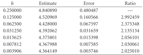
Table 3.1. 1 on Borouchaki and George’s example.
h Estimate Error Ratio
0.250000 4.840890 0.480487 —
0.125000 4.520969 0.160566 2.992459 0.062500 4.428000 0.067597 2.375348 0.031250 4.392062 0.031659 2.135134 0.015625 4.375801 0.015398 2.056101 0.007812 4.367988 0.007585 2.030061 0.003906 4.364149 0.003746 2.025010
in the first chart and
t,
1−1.1 sin(t)2
, t∈
0, arcsin 1 1.1
, (3.2)
in the second chart. Because this boundary curve between the charts is not piecewise linear, triangulations will only approximate the true chart sets.
Consider an approximation of the constant function f =1 on this manifold. Because of the simplicity of this function and the fact that the metric is constant in each chart, the only obstacle to convergence to f in our metric is the convergence of the triangulated sets to the manifold. More specifically,1 over the triangulated manifold will converge to
1 over the approximate manifold at the rate at which the piecewise, linear triangulated boundary converges to the curved boundary. Note that the boundary curve lies inW1,1,
that is, its first derivative is unbounded but bounded in integral. We, thus, expect the convergence of the integrals to be ofO(h), regardless of the degree of polynomial used. Our results inTable 3.1confirm this prediction. Despite the fact that we use a quadrature scheme, precise on polynomials of degree three (called “precision 4 quadrature”), which ordinarily would produceO(h4) convergence, we still observeO(h) convergence to the
value of 4.360403.
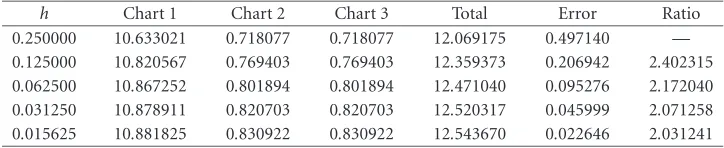
3.2. The unit sphere. We extend the preceding example to the unit sphere. In the case f =1, we know the integral to be 4π, the surface area of the unit sphere. Chart 1 is given byσ1(u,v)=(cos(u) cos(v), sin(u) cos(v), sin(v)), where 0≤u≤π/2 and−π/3≤v≤π/3.
The parametrization of chart 2 is given byσ2(α,β)=(sin(α), sin(β) cos(α), cos(β) cos(α)).
Chart 3 is the same as chart 2, save that the third component is the opposite of the third component in chart 2. The boundary of chart 2 (likewise, chart 3) consists of the boundary curvesv=π/3 (resp.,v= −π/3) of chart 1, transformed into chart 2 co-ordinates, connecting the points (0,π/6), (π/6, 0), (0,−π/6), and (−π/6, 0). The curves |β| =arccos(√3/2 cos(α)) parametrize the boundary in both charts 2 and 3. Observe that these curves have an unbounded derivative which is bounded under the integral sign. Thus, this example resembles the first example in that the bounding curve isW1,1-smooth
and limits the convergence of any finite-element approximation toO(h), as the results in Table 3.2indicate. As before, because these boundary curves areW1,1-smooth, we expect
Table 3.2. 1 on the unit sphere.
h Chart 1 Chart 2 Chart 3 Total Error Ratio
0.250000 10.633021 0.718077 0.718077 12.069175 0.497140 — 0.125000 10.820567 0.769403 0.769403 12.359373 0.206942 2.402315 0.062500 10.867252 0.801894 0.801894 12.471040 0.095276 2.172040 0.031250 10.878911 0.820703 0.820703 12.520317 0.045999 2.071258 0.015625 10.881825 0.830922 0.830922 12.543670 0.022646 2.031241
2 1.5 1 0.5 0 −0.5 −1 −1.5 −2 2
1 0
−1
−2−2 −1
0 1
2
Figure 3.2. Fresnel’s elasticity surface.
3.3. Fresnel’s elasticity surface. This surface (Figure 3.2) appears in the study of op-tics and has the very complicated formx=λcos(u) cos(v), y=λsin(u) cos(v), andz= λsin(v), where
λ=1/
−2
0.965/3−0.935/3cos(u)4+ sin(u)4cos(v)4+ sin(v)4
···cos
arccos
−−0.941/6 + 0.374cos(u)4+ sin(u)4cos(v)4+ sin(v)4
− ···1.309/6cos(u)6+ sin(u)6cos(v)6+ sin(v)6 −1.221 cos(u)2cos(v)4sin(u)2sin(v)2
/··· 0.965/3−0.935/3cos(u)4+ sin(u)4cos(v)4+ sin(v)4 3
+π
/3
+ 0.8
.
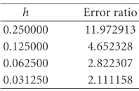
[image:13.468.139.330.193.332.2]Table 3.3. Approximation of1 on Fresnel’s elasticity surface.
h Error ratio 0.250000 11.972913 0.125000 4.652328 0.062500 2.822307 0.031250 2.111158
Because this surface is built from spherical coordinates, we expect and see similar con-vergence results to that of the sphere. Because of the difficulty in working with the com-plicated coordinate maps, direct analysis of these maps has been minimized. The discov-ery of singularities atv= ±π/2 resulted from a numerical sampling script. The alternate parametrizations were constructed indirectly via the application of the above chart map to spherical transition functions. The metric components in different charts were con-structed via finite-difference methods, avoiding differentiation of the above expression. Because we use the same spherical coordinates we used in the sphere example, the charts sets are exactly the same as for the sphere. Finally, the “correct integral,” used to measure the error, results from a fine numerical approximation, given the difficulty of calculat-ing the integral analytically. The results inTable 3.3 were obtained using “precision 3” quadrature.
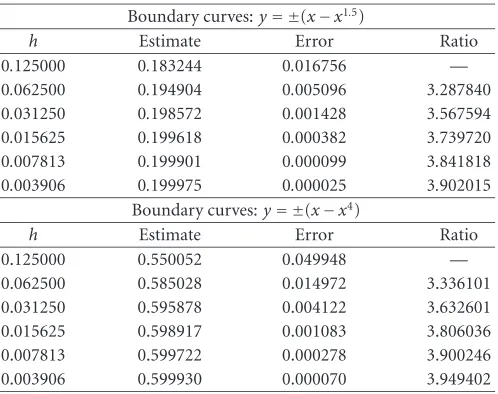
3.4. Boundary convergence whenr=2. For the sake of completeness, we include two toy examples where, like the previous examples, the convergence of the trianglulated boundaries to the boundary curves of the charts dominates the convergence of the in-tegral. In these two examples, however, the boundary curves lie inW2,1 and thus the
convergence progresses atO(h2) (corresponding tor=2 in theJhrterm).
In the first example, we consider a single chart set, given by the area bounded by the curvesyb= ±(x−x1.5). This boundary consists of an upper half and a lower half, both of
which lie inW2,1, but not inC2. The chart map is just the functionΦ(x,y)=(x,y, 0) and
f =1. Thus, the only obstacle to convergence is the boundary. Looping overj=1,. . .,N− 1 whereN≈1/h, we form the rectangle fromxj=j/(N+ 1) toxj+1= j/(N+ 1) and
−(yb(xj) +yb(xj+1))/2 to (yb(xj) +yb(xj+1))/2, divide this rectangle into approximately
N triangles (giving a total ofO(N2)=O(1/h2) triangles), and integrate. Note that this
triangulation method violates the framework of our result in that each vertex of a triangle edge on the boundary does not interpolate aWr,1-segment ofy
b. However, the area of the
difference between this crude triangulation and the one conforming to our framework is ofO(h2) and thus, the convergence rates remain unchanged.
The second example closely resembles the first except thatyb= ±(x−x4). This
bound-ary curves consists of an upper half and a lower half, both of which lie inC∞. However, as predicted by the theorem, we only witnessO(h2) convergence. The results for this
ex-ample and the previous exex-ample appear inTable 3.4.
3.5.Wk,1-surfaces. We examine a case where the smoothness of parametrization map,
Table 3.4. Boundary approximation whenr=2.
Boundary curves:y= ±(x−x1.5)
h Estimate Error Ratio
0.125000 0.183244 0.016756 —
0.062500 0.194904 0.005096 3.287840 0.031250 0.198572 0.001428 3.567594 0.015625 0.199618 0.000382 3.739720 0.007813 0.199901 0.000099 3.841818 0.003906 0.199975 0.000025 3.902015
Boundary curves:y= ±(x−x4)
h Estimate Error Ratio
0.125000 0.550052 0.049948 —
0.062500 0.585028 0.014972 3.336101
0.031250 0.595878 0.004122 3.632601
0.015625 0.598917 0.001083 3.806036
0.007813 0.599722 0.000278 3.900246
0.003906 0.599930 0.000070 3.949402
the metric determinant approximation to slow the convergence. The following two-patch example uses a surface where the map from the chart toR3lies inWk,1, but not inCk.
In the following example, the function being approximated is constant and the manifold is partitioned exactly, so that only the metric approximation term appears in the global convergence estimate.
Each chart set is the square [0, 1]×[0, 1]. The first chart map isσ1(x,y)=(xp+x,y,
xp+x). The second chart map isσ
2(x,y)=((xp+x)(y2−2y+ 2),y−1, (xp+x)(y2−
2y+ 2)). This surface has continuous first derivatives across the mutual edge y=0 in chart 1 andy=1 in chart 2. For a positive integerp, the chart maps have bounded second derivatives. For 1< p <2, the chart maps lie inW2,1, as the chart map have unbounded
second derivatives. Likewise, for 2< p <3, the chart maps lie inW3,1, as the chart map
have unbounded third derivatives. The singularities of these derivatives behave likexp−2
for 1< p <2 andxp−3, for 2< p <3 and occur on the linex=0 in each chart.
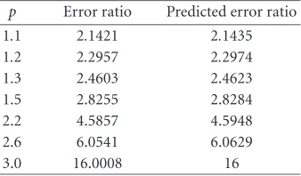
We set f =1. When the chart maps have bounded second derivatives, the inequal-ity (1.4) governs convergence. When the second derivatives are unbounded, a modified version of (1.4) from [19] applies. Forp≥3, we expectO(hk+1) convergence where
poly-nomials of degreekapproximate the chart maps. For 1< p <2, we expectO(hk−1+p)
con-vergence wherek≤1. For 2< p <3, we expectO(hp) convergence fork≥2 andO(h2)
convergence ifk=1. Thus, we expectO(hp) convergence when we use a precision 2
Table 3.5. Approximation of1 onWk,1-surfaces, precision 2 quadrature.
p Error ratio Predicted error ratio 1.1 2.1252 2.1435 1.2 2.2672 2.2974 1.3 2.4123 2.4623 1.5 2.6929 2.8284
2.2 3.9199 4
2.6 3.9860 4
3.0 4.0001 4
Table 3.6. Approximation of1 onWk,1-surfaces, precision 4 quadrature.
p Error ratio Predicted error ratio 1.1 2.1421 2.1435 1.2 2.2957 2.2974
1.3 2.4603 2.4623
1.5 2.8255 2.8284
2.2 4.5857 4.5948
2.6 6.0541 6.0629
3.0 16.0008 16
4. Conclusion
This paper has presented a new framework for measuring the convergence of mesh-based approximation of functions on 2-manifolds. This framework elucidates many of the sub-tle issues of approximation that present obstacles to existing mesh-based approaches. We hope this framework will bring a formalism which unifies our understanding of the many existing, ad hoc approaches to mesh-based approximation on manifolds and surfaces.
References
[1] H. Borouchaki and P.-L. George,Delaunay Triangulation and Meshing. Application to Finite Elements, Editions Herm`es, Paris, 1998.
[2] H. Borouchaki, P. Laug, and P.-L. George, Parametric surface meshing using a combined advancing-front generalized Delaunay approach, Internat. J. Numer. Methods Engrg. 49
(2000), no. 1-2, 233–259.
[3] G. Celniker and D. Gossard,Deformable curve and surface finite-elements for free-form shape design, Comput. Graphics25(1991), no. 4, 257–266.
[4] S. De and K. J. Bathe,The method of finite spheres, Comput. Mech.25(2000), no. 4, 329–345. [5] P. Destuynder and M. Salaun,Approximation of shell geometry for non-linear analysis, Comput.
Methods Appl. Mech. Engrg.152(1998), no. 3-4, 393–430.
[6] C. A. Duarte and J. T. Oden,Anh-padaptive method using clouds, Comput. Methods Appl. Mech. Engrg.139(1996), no. 1-4, 237–262.
[7] ,H-pclouds—anh-pmeshless method, Numer. Methods Partial Differential Equations
[image:16.468.150.319.237.336.2][8] N. Dyn, F. J. Narcowich, and J. D. Ward,A framework for interpolation and approximation on Riemannian manifolds, Approximation Theory and Optimization (Cambridge, 1996), Cambridge University Press, Cambridge, 1997, pp. 133–144.
[9] , Variational principles and Sobolev-type estimates for generalized interpolation on a Riemannian manifold, Constr. Approx.15(1999), no. 2, 175–208.
[10] M. Holst,Adaptive numerical treatment of elliptic systems on manifolds, Adv. Comput. Math.15
(2001), no. 1-4, 139–191 (2002).
[11] M. Holst and D. Bernstein,Adaptive finite element solution of the initial value problem in general relativity. I. Algorithms, in preparation, 2002.
[12] K. Kalik, R. Quatember, and W. L. Wendland,Interpolation, triangulation and numerical inte-gration on closed manifolds, Boundary Element Topics (Stuttgart, 1995), Springer, Berlin, 1997, pp. 395–417.
[13] A. Khodakovsky, P. Alliez, M. Desbrun, and P. Schroder,Near-Optimal connectivity encoding of 2-manifold polygon meshes, Graph. Models64(2002), no. 3-4, 147–168.
[14] K. Lin,Coordinate-independent computations on differential equations, Master’s thesis, Mas-sachusetts Institute of Technology, MasMas-sachusetts, 1997.
[15] J. M. Melenk and I. Babuska,The partition of unity finite element method: basic theory and applications, Comput. Methods Appl. Mech. Engrg.139(1996), no. 1-4, 289–314. [16] F. J. Narcowich, R. Schaback, and J. D. Ward,Approximations in Sobolev spaces by kernel
expan-sions, J. Approx. Theory114(2002), no. 1, 70–83.
[17] J. C. Nedelec,Curved finite element methods for the solution of singular integral equations on surfaces inR3, Comput. Methods Appl. Mech. Engrg.8(1976), no. 1, 61–80.
[18] K. Scully,Finite element approximation over multiple coordinate systems, Phd thesis, University of California, San Diego, 2003.
[19] , OnWk,p-manifolds andWk,p-surfaces for analysis of the convergence of mesh-based approximation, preprint, 2005.
[20] X. Sheng and B. E. Hirsch,Triangulation of trimmed surfaces in parametric space, Comput. Aided Des.24(1992), no. 8, 437–444.
Kevin Scully: The Aerospace Corporation, P.O. Box 92957, Los Angeles, CA 90009-2957, USA