Citation:
Chang, V and Wills, G (2016) A model to compare cloud and non-cloud storage of Big Data. Future Generation Computer Systems, 57. 56 - 76. ISSN 0167-739X DOI: https://doi.org/10.1016/j.future.2015.10.003
Link to Leeds Beckett Repository record: http://eprints.leedsbeckett.ac.uk/1856/
Document Version: Article
The aim of the Leeds Beckett Repository is to provide open access to our research, as required by funder policies and permitted by publishers and copyright law.
The Leeds Beckett repository holds a wide range of publications, each of which has been checked for copyright and the relevant embargo period has been applied by the Research Services team.
We operate on a standard take-down policy. If you are the author or publisher of an output and you would like it removed from the repository, please contact us and we will investigate on a case-by-case basis.
A MODEL TO COMPARE CLOUD AND NON
-
CLOUD STORAGE OFB
IGD
ATAVictor Chang1, Gary Wills 2
1. School of Computing, Creative Technologies and Engineering, Leeds Beckett University, Leeds, UK.
2. School of Electronics and Computer Science, University of Southampton, Southampton, UK.
Abstract
When comparing Cloud and non-Cloud Storage it can be difficult to ensure that the comparison is fair. In this paper we examine the process of setting up such a comparison and the metric used. Performance comparisons on Cloud and non-Cloud systems, deployed for biomedical scientists, have been conducted to identify improvements of efficiency and performance. Prior to the experiments, network latency, file size and job failures were identified as factors which degrade performance and experiments were conducted to understand their impacts. Organizational Sustainability Modeling (OSM) is used before, during and after the experiments to ensure fair comparisons are achieved. OSM defines the actual and expected execution time, risk control rates and is used to understand key outputs related to both Cloud and non-Cloud experiments. Forty experiments on both Cloud and non-Cloud systems were undertaken with two case studies. The first case study was focused on transferring and backing up 10,000 files of 1 GB each and the second case study was focused on transferring and backing up 1,000 files 10 GB each. Results showed that first, the actual and expected execution time on the Cloud was lower than on the non-Cloud system. Second, there was more than 99% consistency between the actual and expected execution time on the Cloud while no comparable consistency was found on the non-Cloud system. Third, the improvement in efficiency was higher on the Cloud than the non-Cloud. OSM is the metric used to analyze the collected data and provided synthesis and insights to the data analysis and visualization of the two case studies.
Key Words
Organizational Sustainability Modeling (OSM); Comparison between Cloud and non-Cloud storage platforms; Real Cloud case studies; data analysis and visualization.
1
Introduction
analyze data. It splits into map and reduce functions, whereby “maps” categorizes the same types of data together and “reduces” then performs the processing of the data to generate the outputs. Often additional algorithms have to be written to ensure smooth processing and transition in the data processing. For example, an optimize function can be written to accelerate the processing time and a visualize function can transform numerical outputs so that users without much technical knowledge can understand the outputs more easily [5]. Big Data in the Cloud offers opportunities for scientists in providing a faster and more accurate technique to analyze their experimental data. At the end of each experiment, terabytes of data can be generated ranging from numerical outputs, the scientific calculations, documentation, images of all kinds (DNAs, tumor and proteins) to datasets, both raw and processed. This will require excellent data processing and management strategies and policies in place, with both automated and manual processing as well as monitoring systems to ensure Big Data services in the Cloud can run smoothly and minimize discrepancies such as fluctuation in network performance, execution time, and termination of services due to job failures. The literature suggests that scientists have used public Clouds to process large scale experiments [4, 6-7]. However, sensitive data such as patients’ records and body images such as tumor and surgery related information, should not be in public domains. All these data should only be within the hospital and not in any public clouds. Hence, the design and implementation of private clouds is essential for biomedical scientists to generate, process, update, archive and store their data. This paper will describe private cloud development for biomedical scientists, whereby high-performance Cloud storage and Big Data processing can be achieved. Our research contributions include:
Direct comparisons between Cloud and non-Cloud platforms about their backup performance.
A model to calculate improvement in efficiency of Cloud systems over non-Cloud systems for biomedical data backup.
Data analysis and visualization.
The breakdown of this paper is as follows. Section 2 describes the related literature. Section 3 explains the system design and implementation. Section 4 presents the OSM model as the metrics for these experiments. Section 5 examines what control measures were in place to ensure an equitable comparison of the non-Cloud and Cloud based back-up systems. Section 6 presents the results of the experiments. Section 7 presents a brief discussion and Section 8 sums up the paper with the conclusion and future work.
2
Related Work
The list of selected literature starts with backgrounds, the process of getting popularity and explanations about the problems associated with the models proposed by the following authors.
Calero and Aguado [8] propose architectures for monitoring Cloud Computing infrastructures and explain their internal and external approaches for monitoring physical and virtual machines. They present monitoring VMs from Cloud consumers point of view and architectures for monitoring in the Cloud. Their approaches are on the full management and monitoring of VMs and performance but do not provide remedies when network outage or latency causes performance downgrade.
Bossche et al [10] focus on IaaS optimization with load prediction. They develop their algorithms based on ARIMA, Holt-Winters and exponential smoothing techniques to achieve renewal contract policies and load prediction. Instead of doing one web log experiment like [9], they adopt 51 real world web application load traces to evaluate their performance although their approaches are not monitoring live systems or applications in real time.
Bower et al [11] propose their high-availability and integrity layer (HAIL) for Cloud Storage. They use mathematical proof and experiments to validate HAIL. In the domain of Big Data in the Cloud, experiments should focus on transferring data across different Clouds. Their results on availability are insightful but they don’t have results for the total time taken, failure rate and performance downgrade caused by latency and large size of files.
Wang et al [12] propose a framework of workload balancing and resource management for Cloud Storage known as “Swift”. They use Swift to discover overloaded nodes and under-loaded nodes in the cluster and then try to make a good balance in all the nodes. A better alternative would be to balance the workload distribution before starting the experiments. Rahman and Rahman [13] propose a Capital Asset Pricing Model (CAPM) for Grid Computing for e-negotiation and resource allocation. However, they do not have continuous monitoring systems or detailed experimental results on data transfer, failure rates and issues caused by latency.
Latch et al. [14] also use relative performance to present their Bayesian clustering software and their key performance indicators are presented as the percentages of improvement. Their work on relative performance needs to be leveraged and adopted by real case studies. Relative performance is defined as the improvement in performance between the old and new service and often the expected outcome is that there is an improvement after adopting new services such as a Cloud Computing service.
The selected literature represents idea and systems that have areas of merits, however, their insufficiencies help focus our research. In as much as; none of the proposed models have investigated performance between a Cloud and non-Cloud system, or how to analyze the data from the Cloud and non-Cloud system. This system should demonstrate Big Data in the Cloud, having experiments on transferring data from one place to another and have the Cloud Storage capacity to offer such a set of services. Our metric (the OSM model) can be instrumental to analyze data, represent the outputs so that the meanings can easily be understood by the stakeholders and system managers, something that is often implicit in the data and difficult for not experts to understand.
3
System Design
This paper describes a real case study in which a new Cloud was designed for biomedical scientists who were required to back up large amounts of data. The new Cloud based back-up service is fast and reliable. We will firstly present the old system (non-Cloud) and new Cloud, based service for a National Health Service (NHS) Trust in the UK. The NHS Trust has invested in the Cloud based service to ensure that all data can be backed-up safely on their systems. The Cloud based service was required to undertake the back-ups, while allowing scientists to carry on with their research and development that produces data that was to be stored safely.
records after each surgery, experiment or simulation. Backup files included data records about patients such as medical records and tumors, detailed descriptions, images and their relationship for each patient. Rapid data growth was observed. New additions of between a few hundred and a few thousand files each week were noted. Hence, a more reliable method to backup all data was necessary. To demonstrate the suitability of the new Cloud based service to effectively back-up the very large datasets (Terabytes of data), large scale experiments were required.
The motivation for the NHS moving to private cloud for big data processing is as follows: First, the stage in implementing the new Cloud based service was to improve the general infrastructure, the University of London Computing Centre (ULCC) decided to carry out a system upgrade which meant their outdated infrastructure and supporting tools would be replaced by new approaches such as cloud storage. Upgrades included fiber optics and high-speed switch network infrastructure to allow advanced experiments to get network high-speeds of up to 10 gigabits per second (GBps). Both the management and scientists would like to use a facility located at the GSTT and ULCC to demonstrate a real collaboration, before the establishment of a new organization, King’s Health Partners. The facilities at ULCC could offer better IT and staff support which could improve the response time and solve the technical problems quicker.
Second, a funding opportunity from the Department of Health, UK was available in 2008. The objective was to design and build a system for providing day-to-day services and improvement of efficiency, including the Cloud Storage solution to process a large amount of data processing daily.
This large scale experiments demonstrates the improvement of efficiency of adopting Cloud over non-Cloud approach and uses a model known as Organizational Sustainability Modeling (OSM) for quantitative analysis. Improvement in efficiency is defined as the difference in the execution time of backup completion between Cloud and non-Cloud services while both services process the same amount of big data job requests. The term ‘jobs’ is used to describe the computer command to backup data from the source to the destination, such as from Guy’s Hospital to St Thomas’ Hospital. Each computer command sends one set of data across two sites, which means that each set of data requires one job to complete backup.
3.1
The non-Cloud Solution
The non-Cloud Storage Area Network (SAN) at St Thomas’ Hospital served the entire GSTT including medical researchers based at Guy’s Hospital. The non-Cloud SAN is formed of four HP storage systems containing a total of 32 terabytes (TB) of storage. Four additional storage servers were added and the total disk storage was expanded to serve up to 64 TB after 2011. This is not classified as a Cloud system, for the following reason: It does not use any virtualization technologies.
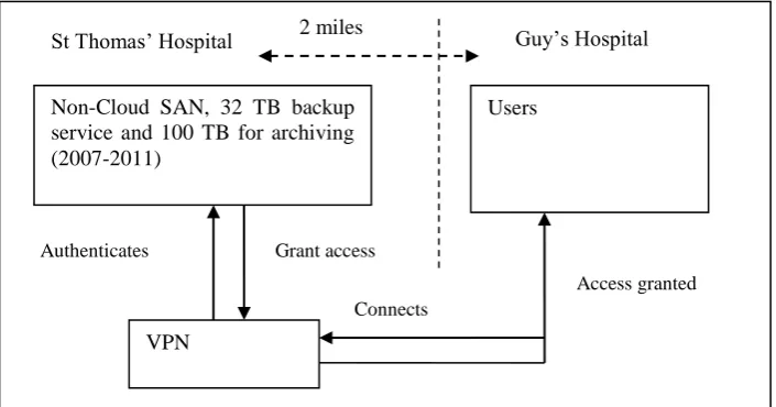
The deployment is not entirely delivered by distributed technologies. Users based at Guy’s Hospital need to get access to a local virtual private network (VPN) server, which then authenticates and connects users to the SAN at St Thomas’ Hospital. The distance between Guy’s and St Thomas’ is 2 miles for network cabling, which has an impact on the network performance. The network speed is 1 GBps (1 GB per second).
3.1.1 The deployment and architecture of the non-Cloud system
There is a control center at the SAN to execute commands for backup services in the
most recent two backup versions are kept. Dependent on the user requests, data backup took place at least once a week. Figure 1 shows the architecture for backup deployment via VPN.
Figure 1: The architecture for backup deployment via VPN
Each job is required to complete the backup process for each dataset. Before beginning to run a batch of jobs, the control centre of the SAN calculates the expected time of completion. A simulation is performed in which all jobs are completed without any failures or incomplete jobs to calculate the expected time of completion. A failed or incomplete job means that the command to send data across the network was unsuccessful and requires another command (job) to send the data again. In other words, it is a simulation to calculate the ideal expected completion time when there are no failed jobs.
When dealing with comparisons of systems involving a large number of jobs, using a simulation method to estimate the incomplete or failed jobs is a common approach [17-18]. A robust backup process should continue without interruptions while keeping the risks (failed or incomplete jobs) to an acceptable rate [17, 19-20]. The backup process in this case study allows thousands of jobs to be completed at once while keeping the number of failed jobs (risk-control rate) under 5% at all times. After authentication, the backup process runs until the completion of the jobs. This backup is a single-direction data transfer, moving data from Guy’s to St Thomas’ Hospital creating an archive of backed up files.
3.1.2 Issues about network performance
Network performance can be subject to the way that the network infrastructure has been set up. Hence, speed of the network, bandwidth and any factors that affect the backup speed should be considered prior comparisons between performance of Cloud and non-Cloud deployment.. The network is expected to lose some speed during the transmission, resulting in lower than 1 GBps transmission rate.
Each Storage Area Network (SAN) has network analytics tools to determine the average actual network speed. There are two types of network speeds: the download and upload speeds. The backup process is dependent on the upload speed, since it sends all the files to the secure SAN storage, to the right storage space, and then archives all the files. Network speed was measured over a period of one year prior to the experiments. The average actual download speed was reduced to 750 MBps during an off-peak period and 550 MBps during a peak period (9-10am, 11am-1pm and between 4-6pm). The average actual upload time is 400 MBps in the off-peak period and 200 MBps in the peak period.
Non-Cloud SAN, 32 TB backup service and 100 TB for archiving (2007-2011)
St Thomas’ Hospital Guy’s Hospital
Users
VPN
Connects Authenticates Grant access
All the backup processes are performed automatically in the off-peak period such as 7 am. During the backup process, occasionally some users required more network bandwidth, which may have caused the lower upload speed being experienced. When such situations happen, the upload network speed, expected execution time and actual execution time for backup completion are recorded.
3.2
The Cloud Solution
From the perspective of healthcare executives, for a Cloud Storage service to be a success and demonstrate better performance than a non-cloud storage service, it must deliver improved efficiency, that is an increase in the time saved by the use of Cloud over non-Cloud services. In the process of doing so, the risk-control should be the same with the improvement of efficiency, so that it can serve as a fair comparison. Additionally, the new Health Cloud platform also provided Bioinformatics services, which offer scientific visualization and modeling of genes, proteins, DNA, tumor and brain images.
3.2.1 System Design stage for Cloud Storage system
The new NHS platform is a Cloud Storage system designed to provide functionality and services for archiving, data storage, data management, automated backup, data recovery and emergency recovery, which are considered as PaaS. The NHS platform was implemented in two phases: (i) design and implementation of Cloud infrastructure and (ii) upgrade from IaaS to PaaS.
The Cloud Architecture design chosen uses two concurrent platforms. The first is based on Network Attached Storage (NAS), and the second is based on the Storage Area Network (SAN). Each NAS device was allocated to a research group to operate independently. All the NAS devices can be joined up to establish a SAN. Each NAS supports individual backups with manual and automated options.
The SAN is a dedicated and extremely reliable backup solution offering a highly robust and stable platform. SAN ensures data is kept safe and archived for a long period of time, and thus is a preferred technology. A SAN can be made up of multiple different NAS systems, so that each NAS can focus on a particular function. Small Computer System Interface (SCSI), an interface and technique used in Storage, is used by SAN to offer dual controllers and dual networking gigabit channels. Each SAN server is built on a RAID system, particularly RAID 10, since it offers good performance like RAID 0, but also has the mirroring capability like RAID1.
A SAN can be built to have 60 TB of disk space, and a group of SAN systems can form a solid cluster, or a dedicated Wide Area Network. Each SAN can feature written and upgraded applications to achieve the following functions:
Performance improvement and monitoring: This allows tracking the overall and specific performance of the SAN cluster, and also enhances group or individual performance if necessary.
Disk management: When SAN system pool is established, it is important to know which hard disks in the SAN support which servers or which user groups.
Advanced features: Advanced features including real-time data recovery and network performance optimization are used.
3.2.2 Deployment Architecture
There were two sites for hosting data: one is at Guy’s Hospital the other is at the University of London Computing Centre (ULCC) to store and backup the most important data. The majority of scientists requiring the backup services are based at Guy’s Hospital and the geographical distance between Guy’s Hospital and ULCC requires two miles of network cabling.
Figure 16 in Appendix shows the Deployment Architecture, and this Cloud-based SAN is made up of several NAS servers. There are five NAS at the GSTT and KCL premises and each NAS is provided for a specific function as follows.
NAS 1 is used for their secure backup for Bioinformatics Group which has the highest storage demands.
NAS 2 provides computational backup for The Bioinformatics Group.
NAS 3 is used as a gateway for backup and archiving and is an active service connecting with the rest. NAS 3 is shared and used by Cancer Epidemiology and Breast Cancer Biology Group (BCBG).
NAS 4 provides mirror services for different locations and offers an alternative in case of data loss.
NAS 5 is primarily used by the Digital Cancer cluster, and helps to backup important files in NAS 3.
There are three NAS systems at the ULCC that offer Cloud and HPC services as follows: NAS 6 is used as a central backup database to store and archive experimental data and
images.
Two further advanced servers are customized to work as NAS 7 and 8 to store and archive valuable data.
NAS 3 and 5 host two digital cancer clusters to backup between each other. Important data can be backed up to both NAS 5 for a local storage version and NAS 8 is provided as added redundancy to deal with disaster recovery. Multiple backups ensure that if one dataset is lost, it can be replaced with the most recent archive (updated daily) quickly and easily. By having a consolidated Cloud solution made up of NAS systems and multiple network routes, performance for backup and archiving services is reliable and has lower rates of risk due to failed jobs.
The four backup servers (NAS 3, NAS 6, 7 and 8 + 1 bioinformatics SAN) implemented in the ULCC offer 160 TB of backup services in Figure 16 in Appendix and they are directly connected (via optical fibers and direct connections) to the 500 TB archiving server where the latest two versions of data records are kept. The entire Cloud Storage Service has automated capability and is easy to use. This service has been in use without the presence of the chief architect (the lead author) for four years without major problems reported. The secondary level of user support at GSTT and KCL (including login, networking and power restoration services) has been available.
3.2.3 The architecture for backup process in the Cloud Storage system
Figure 2: Five routes for the backup process of the Cloud Storage system
Figure 2 shows the entire architecture of the Cloud Storage system and research groups involved in the backup process. A “five-route approach” is adopted for the architecture, where two routes of backup process are dedicated for bioinformatics and three routes of backup process are available for general use for scientists. A simplified representation of the backup process of the NAS systems is provided to help stakeholders understand the processes involved. The Cloud Storage ensures there are five routes for sending large quantities of data records and images over the network to ensure network traffic has no congestion at all times. Each route corresponds to a NAS system at Guy’s Hospital as shown in Figure 2 and handles backup operations in a sequential way. When jobs for the five routes are finished, the backup process is completed.
Each failed job requires an additional three seconds for a system update; which includes displaying an error message to the SAN control center, moving the failed job to the SAN control center and continuing the backup process for subsequent jobs. The main advantage of using multiple network routes relates to the management of failed jobs, which need not use additional time per failed job for status updates. This ensures the backup process is not interrupted by re-handling of failed jobs. The code, status(job), reports the status of the job back to the SAN and status(traffic) reports the status of the network traffic. In the event that any of the five network routes have been congested, the job submissions or requests can choose the next available network route on offer. Each network route is represented as C1, C2, C3, C4 and C5 respectively in Figure 2. To explain the syntax of the algorithm:
continue(status(job)): This means that failed jobs have been detected and the system would like the backup process to go ahead.
stop(status(job)): the job submission or requests are terminated with immediate effect. report(status(job)): the system reports back the job status as a result of completion or
termination.
complete(status(job): the system reporting that the all job requests have been completed without rerunning the failed jobs.
record(status(job): the system reporting completion of job requests to the system manager.
rerun(status(job): the system carries on another process to rerun failed jobs independently. However, the execution time is added to the entire job completion. Cx.status(traffic)): the network status of the network route x. Available for C1, C2,
C3, C4 and C5.
check(Cx.status(traffic)): the system checks the network status of Cx to know whether network traffic is normal without congestion or interruptions by failed jobs.
Cloud SAN, 160 TB backup and 500 TB archiving (2009-2014)
ULCC Guy’s Hospital
Users and architect
All users are authenticated at two sites 2 miles
Bio-infomratics
The main code to manage the backup is presented in Table 10 and Table 11 of the Appendix, whereby the case statements have been used. The algorithm explains that the system checks all the network traffic status of the five routes. All jobs are equally distributed to the five network routes, to reduce the execution time for job completion. If the one in use is congested or interrupted by failed jobs, failed jobs are moved to the next available network route. Additionally, status(job) can be returned as a numerical value, either 0 or 1. When status(job) is returned as 1, it means the job requests have been completed. When it is returned as 0, it means job requests are not yet complete.
To aid the explanation of how the backup process works, here is an example. If there are 10,000 jobs to be carried out, the backup process divides 10,000 into 5, and each route (per NAS system at Guy’s Hospital) can take 2,000 jobs. For example, the first route of the backup sends data records and images to the ULCC Data Center, and there is a 1% risk-control rate, meaning that out of 2,000 jobs, 20 jobs have to be rerun. Instead of spending another 60 seconds (20 x 3 = 60) for the status update, the status reporting can continue while running the second route of the backup process. The backup program continues in this manner for the other four routes, until the completion of the entire process. Hence the time overhead for status updates can be minimized. However, the time overhead to rerun failed jobs remains the same.
3.2.4 Additional advantages of Cloud Storage system
The possibility of network latency can be reduced by taking the “five-route approach” since each route shares the workloads and avoids possible network traffic congestion. With 10,000 jobs (each job contains a data record/image) to manage, network traffic jams network interruptions (such as other non-research departments requiring more network resources, which can interfere with the network backup processes) can be perhaps expected. The code can choose any system to start the backup process in any particular order. This allows the backup process to avoid using a system in high demand as the first starting point. In addition, a Wide Area Network (WAN) optimization service is used in the Cloud Storage. This service reduces network latency, helps avoid blockages in network traffic and keeps the network speed at the optimum level.
3.2.5 A visitto actual versus expected execution time
The use of the Cloud-based system offers a shorter execution time than using the non-Cloud system due to the improved design used to deal with network latency and system reporting. The difference in execution time (both of the actual and expected) between the Cloud and non-Cloud system represents a difference in efficiency however this can be effected by the latency in the network and file sizes used in the back-up process.
4
Organizational Sustainability Modeling: the metric
Non-Cloud and Cloud systems were built serving the backup process for scientific data. Making fair comparisons between the two systems, requires a model that takes the expected outputs, actual outputs and risk-control rates into consideration. The risk-control rate is defined as the rate of job failures which is kept under an acceptable rate and so does not prevent the backup system from terminating or downgrading as a result of job failure. To ensure a fair comparison, it is important to ensure risk-control rate is the same to within 0.1% between Cloud and non-Cloud while making a performance comparison between two systems.
comparisons were performed on each system to record actual execution time. Each experiment corresponded to real usage by end users undertaking backup of their research experiments from 2009-2011. There are other supporting case studies and quantitative analysis conducted by OSM to present the added value offered by Cloud Computing adoption [15-16].
The OSM formula is as follows:
c c
r
-a
r
-e
(1)where
βis the risk measure (gradient of regression),
rc is the risk-control rate,
a is the difference in actual execution time in both systems and
e is the difference in expected execution time in both systems. Interpreting the Beta value, which representing the uncontrolled risk:
If the actual values are higher than the expected values, the beta is less than 1. This can be interpreted as showing that the uncontrolled risk is low and that the Cloud project is not exposed to a high level of volatility.
On the other hand, if the expected values are higher than the actual values, the beta value is higher than 1, meaning that the uncontrolled risk is high. Hence, the project may be exposed to a high level of volatility. Therefore service and technical improvements must be made as soon as possible to justify the benefits of using Cloud. The impacts of inaction may include an under-rating of services, sharp decline in the user community and a discontinuation of services due to unsatisfactory performance.
Three types of metrics are collected for OSM:
The actual return value is the difference between Cloud and non-Cloud systems in the actual total time taken. It can be presented as a percentage.
The expected return value is the difference between Cloud and non-Cloud systems in the expected total time taken. It can be presented as a percentage.
The risk-control rate is the percentage of failed (or incomplete) jobs.
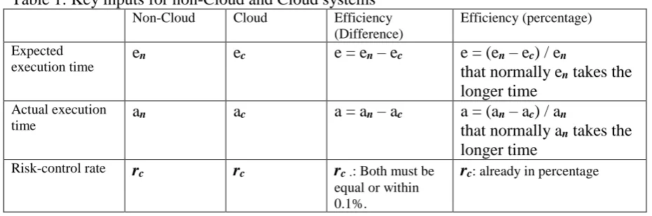
[image:11.595.64.529.614.768.2]Efficiency can be presented as a percentage. Improvement in efficiency is equal to the difference of execution time divided by the execution time of a non-Cloud, which normally takes a longer time than Cloud systems. See Table 1 for explanations.
Table 1: Key inputs for non-Cloud and Cloud systems
Non-Cloud Cloud Efficiency
(Difference)
Efficiency (percentage)
Expected execution time
en ec e = en – ec e = (en – ec) / en
that normally en takes the longer time
Actual execution time
an ac a = an – ac a = (an – ac) / an
that normally an takes the longer time
Risk-control rate rc rc rc.: Both must be
equal or within 0.1%.
4.1.1 OSM Metrics for the non-Cloud and Cloud system
This section aims to explain how the parameters used by non-Cloud Storage and also Cloud Storage systems are relevant to OSM metrics. At the end of the backup process, the system administrator is notified of the result of the jobs, including statistics such as the execution time, number of files backed up and the number of files for which the backup process failed, and the percentage of successful and failed jobs. All these parameters are used in the OSM model and are explained as follows:
Actual execution time: This is the actual time taken to complete the backup process while keeping the rate of failed/incomplete jobs under 5% to ensure controlled risks can be fully managed. Another round of re-running failed/incomplete jobs will be carried out. The actual execution time is the sum of the first round of the backup process and the completion of re-running the backup jobs and includes network latency.
Expected execution time: This is calculated by the network simulator. This is the execution time under ideal conditions where there will be no failed jobs. It can be calculated prior to using the subsystem.
Risk-control rate: This is the controlled risk of running comparisons. The rate of failed or incomplete jobs should be kept under 5%. If the rate is less than 5% then job failures will be reported but will not interrupt the backup process [15]. However, when the rate rises above 5% the entire backup process is terminated and will be restarted on both systems.
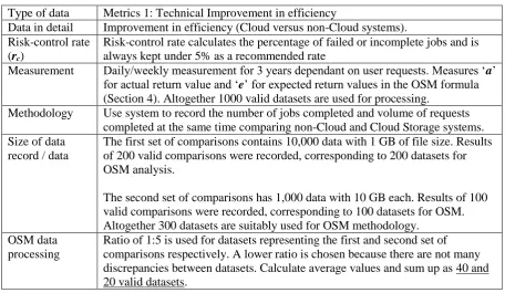
[image:12.595.65.522.448.713.2]A list of data variables, their definitions and explanations is presented in Table 2. Table 2: Overview of OSM Case Study, NHS: Metrics 1
Type of data Metrics 1: Technical Improvement in efficiency
Data in detail Improvement in efficiency (Cloud versus non-Cloud systems). Risk-control rate
(rc)
Risk-control rate calculates the percentage of failed or incomplete jobs and is always kept under 5% as a recommended rate
Measurement Daily/weekly measurement for 3 years dependant on user requests. Measures ‘a’
for actual return value and ‘e’ for expected return values in the OSM formula
(Section 4). Altogether 1000 valid datasets are used for processing.
Methodology Use system to record the number of jobs completed and volume of requests completed at the same time comparing non-Cloud and Cloud Storage systems. Size of data
record / data
The first set of comparisons contains 10,000 data with 1 GB of file size. Results of 200 valid comparisons were recorded, corresponding to 200 datasets for OSM analysis.
The second set of comparisons has 1,000 data with 10 GB each. Results of 100 valid comparisons were recorded, corresponding to 100 datasets for OSM. Altogether 300 datasets are suitably used for OSM methodology.
OSM data processing
Ratio of 1:5 is used for datasets representing the first and second set of comparisons respectively. A lower ratio is chosen because there are not many discrepancies between datasets. Calculate average values and sum up as 40 and 20 valid datasets.
4.2
Comparison with similar methods
term predictions and short-term impact on their QoS and SaaS application. They only use one set of metrics and have experiments conducted over a four-week period rather than the three year period in our approach. Second, Bossche et al [10] develop their algorithms based on ARIMA, Holt-Winters and exponential smoothing techniques to achieve renewal contract policies and load prediction. Their method is an improvement over Calheiros et al [9] and they use 51 different datasets to validate their results. These datasets are not primary datasets like our approach, and they are involved with monitoring the systems in real-time to get their input data. Bower et al [11] propose their high-availability and integrity layer (HAIL) for Cloud Storage. Their results are focused on availability but there are other factors for experiments such as the total execution time, failure rates and performance downgrade caused by latency and large size of files. Wang et al [12] propose a “Swift” framework to discover overloaded nodes and under-loaded nodes in the cluster and then try to make a good balance in all the nodes. OSM makes a good balance of workload distribution before beginning of the experiments and need not worry about this aspect. Rahman and Rahman [13] proposed a Capital Asset Pricing Model (CAPM) for Grid Computing for e-negotiation and resource allocation. They do not have continuous monitoring systems or detailed experimental results on data transfer, failure rates and issues caused latency. OSM can be used before, during and after the experiments for performance comparison, data analysis and visualization.
5
Equitable comparisons
Before comparing Cloud and non-Cloud solution on performance, risk-control rates for both systems must be managed and maintained the same before the comparisons are undertaken. Three factors that can cause failed jobs are identified and solutions for improvement are described. By having better management of these three factors, the number of failed jobs associated with risk-control rates can be reduced. In addition, there are two types of investigations required to identify the impact on the backup process due to network latency and file size. The first investigation aims to understand the relationship between the network latency and risk-control rate. The second investigation aims to understand the relationship between file size and risk-control rate.
As presented previously, each failed job takes an additional three seconds for status update. The backup process still continues and will rerun failed jobs at the end of the first round of the backup process. Information for the failed job system report includes the type of data, the location of the data and the potential reason for failure. For example, if a job to send tumor images across the network for backup fails, then the system can move the failed job to the control center and continue to the next job, and requires three seconds to report the location and information about the tumor images.
The relationship between the number of failed jobs and the risk-control rate is explained as follows. If there are 10,000 jobs for the backup process to complete and 100 of them fail at the first attempt and need to rerun, then the rate of failed jobs is equal to 100/10,000 = 1%. This corresponds to a 1% risk-control rate of sending the 10,000 files for backup.
5.1
Maintaining network speed difference between Cloud and non-Cloud
systems
Network latency, file size and file dependency are three factors that result in failed jobs and downgrade technical performance. Hence a discussion on the effect of variations in network latency and file size, could affect the comparison off the systems.
Both network speed difference should be small (maximum is 10 MBps) to minimize impacts due to network latency and also maintain good quality of data analysis as a result of backup process completion on both Cloud and non-Cloud systems. The term N1 is the only network route used by the non-Cloud system. The process “C1.status(speed)” checks the network speed of the Cloud Storage system taking the first network route as default. Matrix X is created to receive all inputs from Cloud Storage network speeds. The process “N1.status(speed)” checks the network speed of the non-Cloud Storage system. Matrix Y is created to receive all inputs from non-Cloud Storage network speeds. Maxtrix Z is the difference between Matrices X and Y. The process “check(difference)” compares the differences to check if the value is 10 or higher, the backup process will be terminated until the difference becomes smaller. The backup code checks the network traffic condition.
5.1.1 Risk controlled rate: Failed jobs
Based on a whole year of system records, the cause of failed jobs are likely due to the following factors:
1. Network latency: There is inherent network latency in sending a large number of files. Up to 10,000 files are sent to the SAN across the network, for example. This results in delay or interruptions in sending some jobs over the network successfully.
2. The short period of lower upload bandwidth: Some scientists require intense network resources for their work despite being given forewarning about the ‘at-risk’ periods. The short period of lower upload bandwidth and less capacity for network resources may interrupt backup processes. As a result, some jobs fail.
3. Dependency between files: Although scientists are asked to check before the start of the backup process, some file dependencies are not easily spotted. If File B is dependent on File A, and File A is not yet backed up, the backup job for File B will fail if it is queued in front of File A during the backup process. Users are asked to check for file dependency issues between hundreds and thousands of medical records and images. An inspection by the Chief Architect took place prior to the comparisons commencing. File dependency was one of the most common factors affecting risk-control rate in the past few years. If failed jobs happened due to file dependency, failed jobs can run again later. In all the comparisons, failed jobs caused by file dependency were completed successfully after re-running them one more time. Additional time is required when failed jobs occur, including the following overheads:
Rerunning failed jobs: The backup system will run each failed job again at the end of the process.
System status updates: Each failed job takes an additional three seconds to report to the central SAN system for the non-Cloud system. There is only one route and the system cannot go on to backup process without receiving the status update first. Additional delayed time due to network latency – when failed jobs occur, more
can result in further network latency [21-22], thereby increasing the actual time to complete the job.
Since risk-control rate is a controlled risk, it is possible to minimize the risks by the following:
Warning for ‘at-risk’ periods: Sending out emails one week and one day before each experiment helps reduce the number of scientists trying to work on the Storage system during the at the ‘at-risk’ period. Always performing the comparisons in out-of-office hours to ensure the benefits of the higher upload network bandwidth.
File size: 1 GB, 10 GB and 100 GB cover the most common range of file sizes for all user requests. Although the backup on both systems can handle most file sizes, the risk-control rate can vary if the size of each file is different and the total amount of backup files varies. For example, there were 10 x 100 GB files, and 1,000 x 10 GB files and 5,000 x 1 GB files in a particular user request in 2009; all of the backup jobs failed for 100 GB files. The entire backup process was terminated and rerun since the large file size reduced the network performance and prevented other files from being backed up. A lesson learned from this case is to allow one particular file size at a time, such as all files of size around 1 GB, or 10 GB, or 100 GB.
Check dependency between data: Double check with users about data dependency before each experiment. However, if there are 10,000 or more data records and images each time, it is difficult to prevent dependency issues which can either slow down the network or create failed jobs.
5.1.2 Actual execution time
Before the actual running of jobs on both Cloud and non-Cloud systems, the expected execution time is calculated prior to undertaking the actual backup comparisons for Cloud and non-Cloud systems.
Although the ideal network upload speed is 400 MBps, three unexpected events (system updates, users demands, and file size/dependencies) may take the network speed down to 200 MBps, and/or create failed jobs as recorded as the risk-control rate. This explains why upload network speed does not always stay at 400 MBps. Both SAN control centers for non-Cloud and Cloud systems can display the actual execution time of the completion. Synchronizing the comparison of both non-Cloud and Cloud systems is useful, as this makes it easier to work out the difference in execution time for both systems, which corresponds to the improvement in efficiency.
5.1.3 Maintaining network speed during the comparison
Data recovery enabled by snapshots of virtualization technology is not used for comparison. The comparison is based on backup completion across the network. The network speed performance, as well as the need to maintain similar network speed performance to two destinations, becomes the main factor in the backup process.
MBps difference limit. The following is an example to explain how to maintain similar network speeds for both Cloud and non-Cloud services.
The expected upload network speed is around 400 MBps off-peak and 200 MBps on-peak for both systems. A total difference of around 10 MBps means the network speed is operating within 95% of the confidence interval. If there is a difference of more than 10 MBps, the entire backup process to both destinations will halt, freezing execution time. The backup process can resume when there is a speed difference of less than 10 MBps. In all backup experiments for comparisons, network speed difference is checked and maintained within 10 MBps differences to ensure a fair comparison. This is achieved by the process check(difference), which checks network speed differences between Cloud and non-Cloud and the backup process on both Cloud and non-Cloud systems will be suspended until the difference becomes 10 MBps or smaller. The risk-control rate for both systems must be managed carefully and set as close to each other as possible. This can be achieved by:
Synchronizing the comparisons: This can ensure both back-ups start at the same time, and means the management of risk-control rate is handled once rather than twice per experiment.
Network traffic and speed monitoring: The use of tools can measure the network traffic and upload speed time, which can be tracked and presented as graphs. The network monitoring tools can report the upload network speed to two destinations (Guy’s to St Thomas’ Hospital and Guy’s Hospital to ULCC).
5.1.4 Variations of risk-control rate versus network latency (one network route in each system)
There is a direct relation between the failed jobs (represented by the risk-control rate) and network latency. Both Cloud and non-Cloud systems only use one network route for backup in the test. For the purpose of this set of comparisons, 1,000 files each of 1 GB of data in size, to be presented as 1,000 jobs, are used to investigate the difference between risk-control rate and network latency for both Cloud and non-Cloud systems. The network speed is the same between Guy’s Hospital and St Thomas’ Hospital, and between Guy’s Hospital and ULCC, in both cases it is at 400 MBps. Failed jobs can be managed by ensuring a selected percentage of 1 GB data is unable to be sent across the network. See Table 3 for variation in risk-control rate versus network speed.
[image:16.595.96.519.677.768.2]For example, a 1% risk-control rate means that 10 files in every 1GB of data will fail to be sent over the network. Risk-control rates can be varied. Each experiment in risk-control rate variation was performed five times to give an average result of network speed and was performed at 7am (off-peak period) to minimize any interference caused by network users. See Table 3 for results, which show that for every increase of 1% in risk-control rate, the network speed drops by approximately 1% due to network latency. Table 3: Variations in risk-control rate versus network speed due to latency (one network route for Cloud and non-Cloud system)
Risk-control rate (%)
Network speed on Cloud system (MBps)
Network speed on non-Cloud systems (MBps)
Standard deviation (MBps)
0 400.0 400.0 0.0 (both)
0.5 398.1 398.0 0.1 (both)
1.0 396.2 396.0 0.1 (both)
0.2 (non-Cloud)
2.0 392.2 391.7 0.2 (both)
2.5 390.1 389.5 0.2 (Cloud)
0.3 (non-Cloud)
3.0 388.0 387.3 0.2 (Cloud)
0.3 (non-Cloud)
3.5 386.0 385.1 0.3 (both)
4.0 383.9 382.9 0.3 (Cloud)
0.4 (non-Cloud)
4.5 381.8 380.6 0.4 (both)
5.0 379.7 378.3 0.4 (Cloud)
0.5 (non-Cloud)
5.1.5 Variations of risk-control rate versus network latency (five network routes in Cloud versus one network route in non-Cloud)
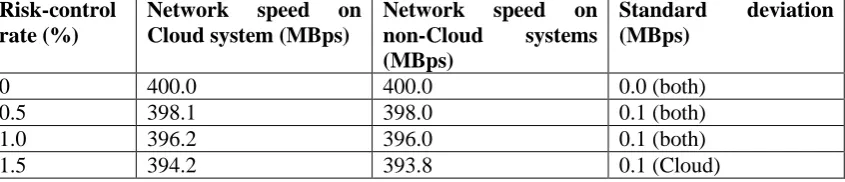
[image:17.595.95.506.345.580.2]This section describes the outcome when five network routes are used for the Cloud system, to determine how network latency affects Cloud systems. The setup is the same as the previous section except all five network routes are available for the backup process. Table 4: Variations in risk-control rate versus network speed due to latency (five network routes on the Cloud systems)
Risk-control rate (%)
Network speed on Cloud system (MBps)
Network speed on non-Cloud systems (MBps)
Standard
deviation (MBps)
0 400.0 400.0 0.0 (both)
0.5 400.0 398.0 0.1 (both)
1.0 400.0 396.0 0.1 (both)
1.5 400.0 393.8 0.1 (Cloud)
0.2 (non-Cloud)
2.0 400.0 391.7 0.2 (both)
2.5 400.0 389.5 0.2 (Cloud)
0.3 (non-Cloud)
3.0 400.0 387.3 0.2 (Cloud)
0.3 (non-Cloud)
3.5 400.0 385.1 0.3 (both)
4.0 400.0 382.9 0.3 (Cloud)
0.4 (non-Cloud)
4.5 399.8 380.6 0.4 (both)
5.0 399.6 378.3 0.4 (Cloud)
0.5 (non-Cloud)
Results in Table 4 show that the network speed on the Cloud system stayed at 400 MBps when risk-control rate was 4% and below. Network speed only dropped slightly (to 399.6 MBps) when the risk-control rate was at 5%. Results from this experiment confirm that the Cloud system with five network routes is not affected by network latency when risk-control rates stay around 5% and below.
5.1.6 Variations of risk-control rate versus file size
backup, and submitting them in the reverse order in the backup process. The file dependency in the test files had been checked consistently to provide different controlled variations in the risk-control rate.
For the purpose of this demonstration, three sets of investigations were used: Set 1: 1,000 files each containing 1 GB of data;
Set 2: 100 files each containing 10 GB of data; Set 3: 10 files each containing 100 GB of data.
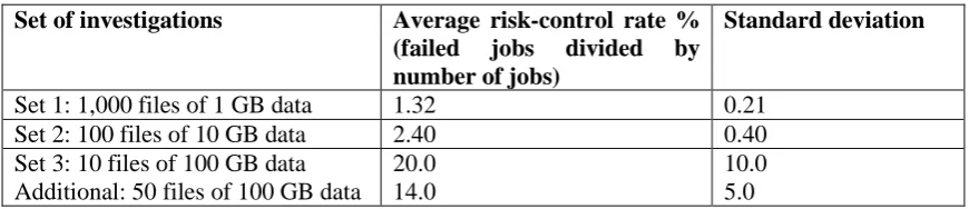
[image:18.595.71.511.303.397.2]These were sent across both Cloud and non-Cloud systems. These three sets of investigations have an equal total of 1TB (1,000 GB) for backup. Each set of investigations is performed five times to get the average results presented in Table 5. The aim of these experiments was to identify the appropriate file size for backup. The 1 GB, 10 GB and 100 GB sets were chosen, since they represent the most commonly occurring file sizes in the user requests between 2007 and 2008. Results will be presented in Table 5.
Table 5: Variations of risk-control rate versus file size
Set of investigations Average risk-control rate % (failed jobs divided by number of jobs)
Standard deviation
Set 1: 1,000 files of 1 GB data 1.32 0.21
Set 2: 100 files of 10 GB data 2.40 0.40
Set 3: 10 files of 100 GB data Additional: 50 files of 100 GB data
20.0 14.0
10.0 5.0
Results in Table 5 show that the risk-control rates are lower than 5% for set 1 and set 2. Therefore file sizes of 1GB and 10 GB can be used for backup comparison. The third set has a 20.0% of failure rate (and a standard deviation of 10%). Since the sample size was small, an additional set of experiments with a larger sample size is carried out- 50 files each with 100 GB of data were used. Again the experiment was run five times and the average results taken. Results show that risk-control rate was 14% with a standard deviation of 5.0. This means backup experiments with 100 GB data are not suitable for OSM methodology due to the higher risk rate of failures.
5.2
Implementation Architecture for the experiments
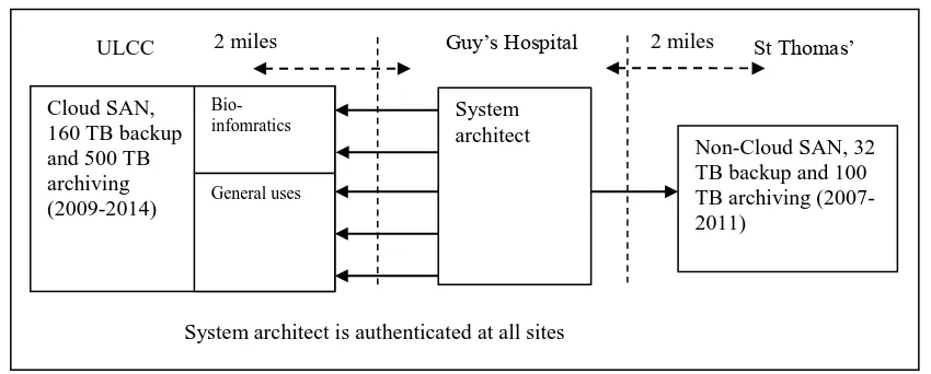
Figure 3: The simplified deployment diagram before each experiment
As a precaution the results from the SAN interface were checked with the log files of the backup process. The aim was to confirm that the execution time and risk-control rates displayed on the third party interface were always consistent with the results on the log files. No discrepancies were found and records of the execution time and risk-control rates were accurate.
5.3
Process for the backup comparisons on Cloud and non-Cloud systems
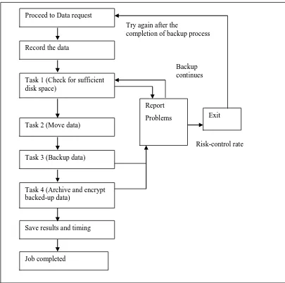
This section focuses on the steps involved with the backup process. The same process is used in both the Cloud and non-Cloud systems. The backup operation performs four tasks. Figure 4 shows the process flow diagram. The backup process is as follows:1. It checks that the destination has sufficient disk space.
2. It begins to move data across the network. This is the point where each experiment has to ensure upload network speed and risk-control rate are consistent at all sites. 3. It backs up all data. Any failed or incomplete jobs are reported. If risk-control rate is
kept under 5% as a recommendation, the entire backup process can continue without interruptions. The SAN control centers can display other information such as the execution time, network speed and number of jobs completed.
4. It archives and encrypts all backed up data. Failed or incomplete jobs will be rerun after the completion of the backup process. If all operations work, the results are saved and actual completion time is recorded.
A script has been written to calculate the improvement in efficiency by comparing the results of the two systems and updating the final values. The following steps correspond to the actions directed from the backup algorithm.
1. Collect results in an old system, put them in Matrix A 2. Collect results in a new system, put them in Matrix B 3. Create a third Matrix (of the same size)
4. Find the difference in each value and store this value in the third Matrix 5. Check values in the third array again
6. Divide each value by 100 (to express as the percentage) and update Cloud SAN,
160 TB backup and 500 TB archiving (2009-2014)
ULCC Guy’s Hospital
System architect
System architect is authenticated at all sites 2 miles
Bio-infomratics
General uses
Non-Cloud SAN, 32 TB backup and 100 TB archiving (2007-2011)
Figure 4: Process flow diagram to show the backup process
The six steps involved help collaborators if they do not perform a weekly backup of experiments, but would like to find out the improvement in efficiency when they have sufficient data. An alternative, not using a script, is to collect data weekly, calculate the difference and present the difference as the percentage of the improvement in efficiency. 5.3.1 Collected datasets for OSM processing
For the purpose of obtaining a meaningful result to investigate the impact of Cloud adoption, three years’ worth of datasets were collected from 2009 to 2011. Each time an approved data request from users was issued, it required a new comparison between a Cloud and non-Cloud systems. In the three years, there were 1,090 approved data requests, which resulted in 1,090 comparisons. The quantity of the datasets for each comparison, ranged from 500 to 2,000 based on the user’s request.
Examinations of the data records showed that not all datasets are entirely suitable for OSM computation due to the file size. Only datasets with file sizes around 1 GB and 10 GB were selected and they are divided as follows.
200 ‘small file’ datasets: 203 data sets each of 1GB in file-size from actual usage data were chosen for the experiment. One dataset represents results of a successful backup of 10,000 files of 1 GB in size on both systems. However, three datasets are out of the range of 95% confidence interval (CI) in the first round of regression, and were therefore dropped. The remaining 200 datasets were used by OSM for the
Record the data Proceed to Data request
Task 1 (Check for sufficient disk space)
Task 2 (Move data)
Task 3 (Backup data)
Task 4 (Archive and encrypt backed-up data)
Save results and timing
Report
Problems
Job completed
Exit Try again after the
completion of backup process
Risk-control rate Backup
comparison. This means there are 10,000 observations performed 200 times for statistical analysis.
100 ‘large file’ datasets: 102 data requests were approved. However, two datasets are out of the range of 95% CI in the first round of regression and only 100 datasets are selected for OSM analysis. In other words, 100 valid experiments (1,000 files of 10 GB data) were performed to support OSM methodology. It also means there are 1,000 observations performed 200 times for statistical analysis.
5.3.2 Calculations of the expected execution time for the non-Cloud system
To demonstrate a case for the expected execution time calculations, there are 10,000 files each of 1 GB in size (or as close to 1 GB as possible), and there is a total of 10,000 x 1 = 10,000 GB of data to be backed up. The upload speed is 400 MBps, or 400 MB (or 0.4 GB) of data is moved across the network every second during the off-peak hours.
The total time for the backup is equal to the total amount of data divided by the upload speed. In the best-case backup completion scenario where risk-control rate is set at 0% (the ideal situation), the calculations are as follows.
Expected execution time to complete backup of user’s experiments
= total size / upload speed = 10000 / 0.4 = 25,000 seconds = 6 hours, 56 minutes and 40 seconds
The occurrence of failed jobs adds to the risk-control rate and the additional time allocated for it. If the risk-control rate is 1%, it means 10,000 x 1% = 100 files that need to be backed up again (or 100 new jobs for full completion, where each data file has 1 GB in size).
Additional system reporting time = Number of failed jobs x additional backup time = 100 x 3 (each failed job needs 3 seconds for status update)
= 300 seconds
Job completion time to rerun failed jobs = 100 / 0.4 = 250
Additional time due to network quality: 1% risk-control rate can result in 1% drop in the network quality of service (QoS). This means that an additional time will be taken for backing up of 25,000 x 1% = 250 seconds.
Total additional expected time = 300 + 250 + 250 = 800 seconds = 13 minutes and 20 seconds
Expected execution time to complete back up of user’s experiments with 1% risk-control rate = 6 hours, 56 minutes and 40 seconds + 13 minutes and 20 seconds = 7 hours and 10 minutes. Expected execution time in regard to risk-control rate can be calculated in this way and is all recorded in seconds.
5.3.3 Calculations of the expected execution time for backup completion
This section describes how to calculate expected execution time for Cloud Storage. The same parameters are used: 10,000 jobs (transferring 10,000 files of 1 GB) are measured and 400 MBps is the upload network speed for the experiments. Although the Cloud Storage system has five routes for the backup, each route is taken one at a time, and it makes no difference for expected execution time if there are any failed jobs.
= 10000 / 0.4 = 25,000 seconds
= 6 hours, 56 minutes and 40 seconds This is the same as non-Cloud SAN time
Additional time due to risk-control rate: The Cloud storage system can save time compared to the non-Cloud system when dealing with failed jobs. If the risk-control rate is 1%, the additional time for system status reporting is not required, since failed job status can be reported while running jobs on another network route. This then saves 100 x 3 = 300 seconds. Additional time due to network quality: There are five route approaches. This means that when there are failed jobs, the network quality of service is unaffected. It does not take the overhead of an additional 1% of lower quality of service time, which is 25,000 x 1% = 250 seconds.
Job completion:
100 failed jobs need to be rerun and the expected time to rerun failed jobs = 100 / 0.4 = 250 seconds
Expected execution time to complete experiments with 1% risk-control rate = 6 hours, 56 minutes and 40 seconds + 250 seconds = 7 hours and 50 seconds
The Cloud Storage system is 300 + 250 = 550 seconds faster than the non-Cloud system in terms of expected execution time.
The expected return value can be presented as a percentage. This is simply the time
difference of 550 seconds divided by the total execution time of the non-Cloud system of 7 hours and 10 minutes in Section 5.3.2.
Expected return value = 550 / 25,800 = 2.132%
The improvement in efficiency for the expected return value is 2.132% for the 1% risk-control rate case.
6
Experiments and results
Mortier [24] examined network traffic engineering and how it could affect network performance. Experiments on two large cluster systems were performed sending data across a single network. He demonstrated that a bottleneck could occur leading to delays if there was only one network route. He proposed multiple network routes. In his experiments with multiple network routes, there was very little delay since network routes were always available to complete jobs.
In these experiments, the Cloud system has five network routes to ensure backing up data across the network can be successful with good network traffic flows. To demonstrate the impacts of network traffic routes in regard to risk-control rates, two sets of experiments were conducted. The purpose of the first set was to compare backup completion on non-Cloud and Cloud systems, where both use only a single network route for backup. The second set compared both systems, where the non-Cloud system uses one network route and the Cloud system uses five network routes.
6.1
Between Cloud and non-Cloud systems
the job failures and the system can proceed onto the incomplete job handling with errors reported. This means the backup process can be interrupted the least. Figure 5 shows that the expected execution time between Cloud and non-Cloud and how the non-Cloud always has longer execution times than the Cloud due to additional time needed for dealing with job failures, network latency and system reporting. The y-axis represents the execution time for job completion (of migrating 1,000 of files of 1 GB data) in seconds and x-axis represents the number of experiments performed. Amongst all 40 experiments performed, there is a good match of the difference between Cloud and non-Cloud systems.
Expected execution time between Cloud and non-Cloud
24800 25000 25200 25400 25600 25800 26000 26200 26400 26600 26800
1 3 5 7 9 11 13 15 17 19 21 23 25 27 29 31 33 35 37 39
Exe
cut
ion
tim
e
(s
ec
s)
Total expected sec (non-Cloud) Total expected sec (Cloud)
[image:23.595.77.486.185.425.2]Number of experiments
Figure 5: Expected execution time between Cloud and non-Cloud
Figure 6 shows the actual execution time of Cloud and non-Cloud system where the actual execution time for the Cloud is shorter than the non-Cloud in 40 experiments. The overall trend is fairly consistent with an average of 1,550 seconds less than the non-Cloud systems.
Actual execution time between Cloud and non-Cloud
24500 25000 25500 26000 26500 27000 27500
1 3 5 7 9 11 13 15 17 19 21 23 25 27 29 31 33 35 37 39
Exe
cut
ion
tim
e
(s
ec
s) Total
actual (non-Cloud)
Total actual sec (Cloud)
Number of experiments
[image:23.595.76.486.503.728.2]6.2
Expected and actual execution time for the Cloud system
Figure 7 shows the expected and actual execution time for the Cloud, where there is more than 99% consistency between all the execution times in 40 experiments. This set of results also validates the system strategies to migrate to Cloud Computing since there is a high consistency in the performance between the predicted and actual performance. The use of OSM helped to achieve high consistency since impacts such as network latency and job failures can be minimized.
Expected and actual executine time for the Cloud: more than 99% consistency
25430 25440 25450 25460 25470 25480 25490 25500
1 3 5 7 9 11 13 15 17 19 21 23 25 27 29 31 33 35 37 39
Exe
cut
ion
tim
e
(s
ec
s)
Total expected sec (Cl oud) Total actual sec (Cl oud)
Number of experi ments
Figure 7: Expected and actual execution time for the Cloud
[image:24.595.74.511.180.404.2]6.3
Expected and actual execution time for the non-Cloud system
Figure 8 shows the expected and actual execution time for the non-Cloud. There is a huge discrepancy between both sets of values. Results are more similar to Figure 5 and Figure 6 rather than Figure 7. The main reason is the job failures which mean more time is needed to clear the incomplete tasks, rerun failed jobs and waits due to network latency caused by job failures.
Expected and actual executine time for the non-Cloud: a large difference
26000 26200 26400 26600 26800 27000 27200
1 3 5 7 9 11 13 15 17 19 21 23 25 27 29 31 33 35 37 39
Exe
cut
ion
ti
m
e
(
se
c)
Total actual (non-Cloud)
Total expected sec (non-Cloud)
Number of experiments
[image:24.595.73.514.540.749.2]6.4
The comparisons between risk-control rate, expected and actual rate of
return by using OSM
OSM is the model used to measure the effect of the risk-control rates, which is represented by the difference in actual execution time of job completion between the Cloud and non-Cloud systems. Expected execution time can be calculated by using formulas and descriptions above. All the 40 experiments for both Cloud and non-Cloud systems have their respective 40 sets of values for risk-control rate, expected and actual execution time. Figure 9 shows that the actual rate of return has a highest percentage between 5% and 6%, and the expected rate of return has between 3.5% and 4.2% of improvement. The risk-control rates in all the experiments were kept 2% and below for all 40 experiments. Using the Cloud solution, there are higher rates of efficiency improvement.
Risk-control rate, expected and actual rate of return of using OSM
0 1 2 3 4 5 6 7
1 3 5 7 9 11 13 15 17 19 21 23 25 27 29 31 33 35 37 39
Pe
rc
ent
ag
e
%
Risk-control (%)
Expected (%)
Actual (%)
[image:25.595.75.518.238.465.2]Number of experiments
Figure 9: Process flow diagram to show the backup process
6.5
Experiment 1: OSM analysis and discussions using files 1 GB in size for
data backup
6.5.1 Key results and interpretation
[image:26.595.71.513.98.226.2]Key statistical results and analysis for OSM is presented in Table 6.
Table 6: OSM experiment 1 - Key statistics for calculating improvements in efficiency
Parameters Value Parameters Value
Beta
68.67% of risks: external and 31.33% of risks: internal
0.51863 Durbin-Watson
Pr > DW (negative autocorrelation: maximum of 1 in favor of OSM) First order test for p-value
1.0637 0.9992
0.0008 Standard Error 0.1103 Regress R-Square (99.99% C.I) 0.6867 Mean Square Error (MSE) 0.0017 Regress R-Square (95% C.I) 0.9007
Interpretation of output results is as follows. The three key statistics:
Standard error is the standard deviation of the sampling distribution of the mean. It can be interpreted as a statistical term that measures the accuracy with which a sample represents a population [25] and is equal to 0.1103. The low value suggests the results of most of the metrics are close to each other and have few instances of outline data points. In other words, there is a high consistency between all metrics due to a good management of risk-control rate.
The first order Durbin-Watson is used to test the autocorrelation in the regression. As the Durbin-Watson is greater than one (1.0637), there is consistency in the data when run only once, over the time period of the experience.
Beta is the risk measure which indicates the extent of uncontrolled risk. Beta is 0.51863 and is considered a medium-low value. This low value suggests the project is subject to less volatility of uncontrolled risk.
In addition:
The low value (0.0017) of the Mean Square Error (MSE) means there is a very high consistency between actual and expected return values.
The result for main regression is 0.6867. Regression for 95% CI is optional and the result is 0.9007. It also means 68.67% of risks are from the external factors and 31.32% of risks come from the internal factors. Confirmed by the project lead, external risks include the following:
1. Delay in data request process approval: Each time the GSTT data committee waited for a period of time and approved several requests. The delay would result in running several comparisons in one day. In an ideal situation, each experiment should start fresh and there would only be one experiment a day in order to eliminate other possibilities affecting performance, but it is not feasible that way in the actual IT operations.
2. Network resource fluctuation in other departments: Although the comparisons always took place in off-peak periods, there were a few situations where more network resources were required. For example, scientists and surgeons in other departments occasionally do their work during ‘at-risk’ periods (despite warnings that this would interfere with the comparisons).