Theories and Tests for Bubbles

Theories and Tests for Bubbles

Sirnes, Espen

University of Tromsø

1997

bubbles

av

Espen Sirnes Larsen

Hovedfagsoppgave i Sosialøkonomi

Norges

Fiskerihøgskole

Universitetet

i Tromsø

Veileder: Derek J. Clark

1. INTRODUCTION 6

1.1 Notation in the theoretical part (prior to chapter 3) 8 1.2 Notation in the empirical part (chapter 3 and further) 9

2. BACKGROUND: THE OVERLAPPING GENERATIONS MODEL 10

2.1.1 Definition of the functions 10

2.1.2 Savings and the interest rate 11

2.1.3 Diamond equilibrium and dynamic efficiency 14

3. THEORIES ABOUT BUBBLES 17

3.1 Introduction 17

3.2 The fundamental price in the stock market 18 3.3 A Model with an explicit utility function 20

3.4 Rational bubbles 22

3.4.1 If the transversallity condition does not hold 22

3.5 Dynamics 24

3.5.1 The investment effect 26

3.5.2 The arbitrage effect 28

3.5.3 Dynamic efficiency and diamond equilibrium 30

3.5.4 Trajectories 31

3.5.5 If the bubble asset paid dividends 32

3.5.6 Bubbles, dynamic efficiency, Pareto efficiency and money 32

3.5.7 Stochastic bubbles 33

3.5.8 Stochastic bubbles in general equilibrium 34

3.6 How bubbles can arise in a not fully rational market 35

3.6.1 A two-traders model 37

3.6.2 Market biases 38

3.6.3 Overreaction 39

3.6.4 A model with feedback 41

4. TESTING FOR BUBBLES 47

4.1 Shiller’s variance test. 48

4.2 West specification test 50

4.2.1 Introduction: A simple test 50

4.2.2 The information set 51

4.2.3 The model 52

4.2.4 Logarithmic difference 55

4.2.5 Calculation of the variance-covariance matrix 56

4.2.6 The test statistic 57

4.2.7 Diagnostic tests 58

4.2.8 Proposition: A modification of the test in the case of a small sample period 59

4.2.9 Comments about the test 59

5. EMPIRICAL RESULTS 61

5.1 General 61

5.1.1 The data 61

5.1.2 The Sub-indexes 64

5.1.3 Stationarity 65

5.2 Shiller’s variance test 66

5.3 West’s specification test 67

5.3.1 Diagnostics tests 67

5.3.2 Statistical deviation from West’s method 69

5.3.3 The dividend process 69

5.3.4 The simple test 71

5.3.5 The two and four lags model, differenced and undifferenced, with one sample 72

5.3.6 The two and four lags model, differenced and undifferenced, with four samples 73

5.3.7 The log-normal random walk model 75

5.4 Discussion 76

5.4.1 The test statistics 76

5.4.2 The proposed modification of the test 78

5.4.3 Conclusion 79

6. CONCLUDING REMARKS 81

6.2 Non-rational bubbles 82

6.3 The situation in Norway and implications for the global financial markets 83

7. APPENDIX 85

7.1 Derivation of the specification constraint vector R 85

7.1.1 The undifferenced case 85

7.1.2 The differenced case 87

7.2 The companies used in the samples 89

7.3 The estimated parameters 90

7.3.1 The original model 90

7.3.2 The sub-index tests: 91

7.4 The ADF tests 93

7.5 Test statistic for the individual sub-indexes: 96

1. Introduction

In this dissertation I will explain some of the theory about bubbles, and especially bubbles in

the stock market. The intention is to give a presentation of the concept of bubbles in general

and how it may affect the Norwegian economy. I will then make an empirical investigation,

aiming to reveal whether there are signs of bubbles in the Norwegian stock market or not.

Finally, some conclusions will be drawn on the basis of this. Before explaining the contains of

this dissertation any further, I believe it is appropriate to suggest an exact definition of what a

bubble is for readers that are unfamiliar with this term:

A bubble is the component of an assets price that is expected to pay no dividends

If the buyer is rational the investment in this asset is done purely in the belief that the price

will be higher when the asset is sold. The fundamental price (the asset price less the bubble) is

calculated as the expected future dividends in infinite time.

The topics of the different chapters are as follows: Chapter two will be a presentation of the

theory necessary to derive the concept of rational bubbles in the economy. I will here explain

the Overlapping Generations Model. Important concepts will be presented, and then used in

chapter three. In chapter three , I will present bubbles that are rational and not completely

rational bubbles. Rational bubbles are the easiest to analyse, because we can infer something

about which solutions will be beneficial for people in the economy, and thereby limit the

possible outcomes. I will derive the theory used to explain rational bubbles and how a stable

equilibrium can occur. The theory will be generalised to include bubbles that have a chance of

bursting, stochastic bubbles. To give a full perspective of what bubbles are, I will give some

examples during the presentation.

In the theoretical chapters, much work has been devoted to make the concept of bubbles more

accessible, without compromising accuracy. The main reason for the inaccessibility, was that

much literature on bubbles were found to make «leaps» in the theoretical presentation1. It has

1

therefore been necessary to «fill inn », so that there would be no missing parts in the

argumentation.

Of non-rational bubbles, there is to my knowledge no precise theory about. I have therefore

only discussed this in a more general manner. In the part of this chapter that concern

non-rational bubbles, there will also be described some research that investigates irnon-rationality in

the market.

After the theory is presented, in chapter four, I will give two examples of ways to test for

bubbles which I will perform on Norwegian data in the period 1976 to 1997. The tests that

will be applied are Shiller's variance test and West's specification test. I have modified West's

test, the most extensive of the tests, to accommodate the short span of the data set.

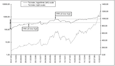
In chapter five the results will be presented. It was unfortunately impossible to get data from

earlier than 1977, so the results can be criticised as suffering from a small sample. Yet, I do

not believe that to be a problem in this dissertation since some of the aim of the empirical part is to show how the tests can be performed and analysed, in particular West’s test with my modifications. The data consist of time series from thirty companies registered at Oslo

Bourse.

A general discussion will be done in chapter six. Conclusions based on the findings in the test

and the theory will be presented. The theoretical results discussed in chapter three is used to

derive implications for the economy in general and specifically how bubbles affects the

1.1 Notation in the theoretical part (prior to chapter 4)

a: The discount factor (a1 1 r)

At: A factor that reflects productivity within a firm

Bt: The aggregate value of the bubble at time t

bt: The value of the bubble in per capita terms at time t

c1t: Consumption of the young at time t

c2t: Consumption of the old at time t

ct: Consumption at time t

dt: The dividend of an asset at time t

et The error term of the bubbles value at time t in the stochastic bubble model

f(k): The per capita production function at time t.

It: The information set at time t, consisting of all information available to the market at this time

Kt: The capital stock at time t

kt: The per capita capital stock at time t

L: The initial population - the population at time t: L(1+n)t

M: The number of bubble assets

mt: The number of assets purchased at time t

n: The population growth rate

Ot: Bonds issued by a firm

pt *

: The fundamental price of an asset at time t (a particular solution to equ. (1))

pt: The price of an asset at time t

r: The short term risk-free rate of return.

s(...): The per capita saving function.

~

u_jt The stochastic error term of the expected return at time t of asset j

wt: The wage at time t

y: The exogenous real endowment of the individual

: The individual discount rate

1.2 Notation in the empirical part (chapter 4 and further)

a: The discount factor (a1 1 r) A: The aggregated data set

bt: The bubble component of the market price

: Auto regression parameter for the price process dt: The dividends of an asset at time t

: Auto regression parameter for the dividend process

Ft The information set available at time t (Bond and Thaler (1985) model)

Ft m

The information set used by the market at time t (Bond and Thaler (1985) model)

ht(): The vector of the auto regression equations

It: An information set at time t, consisting of all information available to the market at this time

Ht: An information set consisting of earlier dividends and a constant, a subset of information set It.

k The number of parameters in a model

m: Constant in the price process : Constant in the dividend process pt

*

: The fundamental price of an asset at time t

pt: The market price of an asset at time t

: The vector of auto regression parameters R The constraint equation in the simple case

R(): The vector of the constraint equations

~

Rit: The return of asset j at time t (Bond and Thaler (1985) model)

RRRS The restricted residual sum of squares, the sum of squares resulting when there are restrictions

imposed on the parameters

S: The sum of the auto covariance matrices.

URRS The unrestricted residual sum of squares, the sum of squares resulting when no restrictions are

imposed on the parameters

ut: The error term of the arbitrage equation

V: The variance matrix

vt: Error term for the dividend process

wt: Error term for the price process

Xn Sub-index n, n=1,2,3,4

zt: The error of the expected sum of future dividends caused by misspecification of the information set It

2. Background: The Overlapping Generations model

The Overlapping Generations Model (OLG) was introduced by Allis (1947), Samuelson

(1958) and Diamond (1965) (Blanchard & Fischer 1994). In the simplest model, the society

consists of two generations, the young and the old, and two sectors, individuals and firms. The

young produce and saves capital for the next period when they are old. Consequently the

young are the workers and the old the capital owners at any time. The economy is a closed

one, with markets that work efficiently. The model was developed by Diamond, building on

work by Samuelson. This kind of two-generation economy is therefore called a Diamond

economy.

2.1.1 Definition of the functions

The individuals have a utility function u(ct) where c1t is consumption for the young and c2t for

the old at time t . Since they live in two periods, they have the total discounted utility during

their life of:

( 2.1) u c

   

1

 



 where 0, u  

 

 

Utility is increasing, but at a decreasing rate. It also assumed that the utility function is

separable across time (one function for each period). This ensures that the goods are normal.

The individuals earn a wage wt during the first period, some of which is spent on savings

stwhich pays the interest rate of rt+1 next period, and the rest on consumption. What is saved in the first period is the capital stock next period. The population is L in period t=0 and grows

at a rate (1+n). In this model, the growth of the population and the growth of the economy are

equivalent terms.

It is assumed that firms act competitively and that the production function for all the firms

together at time t can be characterised as Yt F K L









 ,  1 , which is a function assumed

to be homogenous of degree one. Kt is the total amount of capital invested last period and

therefore the capital stock at the beginning of period t (so the capital this period equals

account of. If capital per worker,





1 , then output per worker is:

 



_



_





_

_

f k F K L n

L n F

K L n t t t t t t               , , 1

1 1 1 . The last equality holds because the function is

assumed to be homogenous of degree one. This production function is assumed to be strictly

concave and to satisfy the Inada conditions:

( 2.2) f

 

 

 

Since the function is strictly concave, we have that f

 

2.1.2 Savings and the interest rate

Under these conditions an individual born at time t has to solve the following problem

( 2.3) _cmax_c u c

   

t t t

t

1 2 1 1

2 1 1 , _            

subject to the budget constraints:

( 2.4) c_1t  s_t w_t and c_2t1  





The first condition is that the wage of the young must equal consumption and savings. The

next is that the capital gains and the savings of the old equals consumption. The first order

condition for an interior maximum is:

( 2.5) 

  

  

 

 

u ct r u c

t t

1

1 2 1

1

1  0

Using the budget constraints and differentiating with respect to savings, wage and the interest

rate yields

 

 

 



  



  

          

 

      

u c_1t dw_t u c_1t ds_t u c2t 1 drt 1 rt 1 u ct dst rt u c t s drt t

2

2 1 1 2 1 1

1 1

Which implies a saving function s(wt,rt+1) with these properties:

( 2.6)





 





  

  

ds dw

u c

u c r u c

t

t

t

t t t

       _  _  1 1 1 0 1 1 1 2 2 1   and

( 2.7)

  



 





  

  

ds dr

u c r s u c

u c r u c

t

t

t t t t

t t t

                    1

2 1 1 2 1

1 1 2 2 1 1 1 1 0 

As we can see, saving increases with the wage. We know that the income effect will increase

consumption in both periods. There are no inferior goods, since we have assumed that the

utility function is separable. An increase in the wage, keeping the interest rate constant, must

therefore be spent on both more consumption in period one, and more savings.

The interest rate effect is ambiguous due to the presence of both income and substitution

effects. The income effect is in this case negative in contrast to the positive effect when wage

is increased. The income effect of an increased interest rate increases consumption in both

periods as mentioned before, but since the available resources in the first period (the wage) do

not change, this has a negative effect on savings. This can be derived as follows: a higher

interest rate increases consumption by dc1t>0, but the wage does not increase, dwt=0. If we

use this and differentiate the budget constraint in the first period in ( 2.4) we get

dst  dct1 0. The first term in the numerator of ( 2.7) can therefore be interpreted as the

income effect and the second term the substitution effect. The substitution effect is positive on

savings since an increase in the interest rate makes consumption in next period cheaper so

savings are increased.

It is difficult to know which effect is the strongest, but if the elasticity of substitution between

the two periods is independent of the interest rate, savings will be too. ( 2.5) may be rewritten

in terms of the elasticity of substitution between the two periods t,as:

( 2.8)







 



 

1

1 1 1

By using the budget constraints and rearranging we get s_t  c_1t_t. This is independent of the interest rate if the elasticity of substitution is independent of it.

This is basically the only thing we can know for sure of the effect of the interest rate on

savings in this model. In a more complicated and perhaps realistic model where individuals

earn a wage in all periods, Blanchard and Fischer argue that the interest rate has positive

effects on savings. I will however not explain this model any further, since it is the model

described previously that will be used in relation to the theories about bubbles.

To see why the influence of the interest rate on savings is important for a theory about

bubbles, we must turn to how firms behave. Firms hire labour and capital up to the point

where the costs equal the marginal product of the input factor, which implies that:

( 2.9)

 

 

 

w f k k f k dw

dk

r f k dr

dk

t t t t

t

t

t t

t

t

     

   

0

0

The rate of interest equals the marginal product of capital because people are considered risk

neutral, there are no implementation costs and all capital can be consumed. According to the

earlier assumptions of the production function, the wage increases with the capital stock and

the interest rate decreases. The two effects are compared in steady state.2

In steady state, the dating of the variables can be ignored, so the effect of the capital stock on

savings in that case can be written:

( 2.10) ds

dk ds dw

dw dk

  0 and ds

dk ds dr

dr dk

  _0.

In the more complicated model mentioned earlier, interest rates had positive effects on saving.

If this is the case, then the effect of an increased capital stock works different ways through

interest rates and wage. For a bubble to arise, the sum of the two effects must be positive and

2

more than (1+n), because savings must increase faster than capital. If dk

ds  1 n, savings in

one period will be exceeded by capital in per capita terms the next period. The reason for this

is that the growth in the economy reduces the per capita earnings next period. This will be

explained more thoroughly in the next chapter.

2.1.3 Diamond equilibrium and dynamic efficiency

If there is no bubble in the economy, net savings (savings less the present capital stock) must

equal investment:

( 2.11) K_t1K_t  L









In per capita terms, and eliminating the present capital stock we can write the Diamond

equilibrium as:

( 2.12)









This is the condition of equilibrium in the goods market if there are no bubbles. The reason it

is called the Diamond equilibrium here, is to stress just that. The term «Diamond equilibrium»

is used when an economy in which bubbles can possibly arise, does not actually exhibit a

bubble.

In the OLG model the competitive equilibrium may not be Pareto efficient. This situation is

called dynamic inefficiency. A Diamond economy is dynamically inefficient if the capital

stock is in excess of that consistent with the golden rule since Pareto improvements are

possible. The golden rule is that the marginal product of capital equals growth, f k( ) =n. If



f k( ) <n the capital stock is in excess of this golden rule level, because the marginal product

of capital is a decreasing function its argument. The reason Pareto improvements are possible

can be derived as follows.

The capital stock and the production function in period t determine how much can be used to

invest in capital and how much can be consumed next period:

Dividing this by the population at time t, noting that k_t1





L n n

t t 

  

1 1

1 1

( + ) ( )

K

L n

t t 1

1

( + ) and rearranging, yields the equation in per capita terms:

( 2.14) k_t  f k( )_t  (1 n k) _t1c_t

In steady state, capital accumulation will be:

( 2.15) k* f k( *) (1 n k) *c* or f k( *)nk* c*

Differentiating:

( 2.16) dc

dk f k n

*

*

*

( )

  

If the marginal product of capital is less than the growth, f k( )n, a given permanent

decrease in the capital stock will increase consumption in all periods but the last. That

consumption in the last period will decrease can be seen from equation ( 2.16). If f k( )n, consumption and the capital stock is negatively related, so a decrease in the capital stock will

increase consumption. In the last period however, there will be no future period to invest in,

so consumption will decrease: differentiating equation ( 2.14) at time T with respect to the

permanent change in capital k, noting that kT+1=0 yields:

 

dc

dk f k

T

*

*

   1 0. But since

period T is in the infinite future, this decrease in consumption due to a reduction in the capital

stock can be ignored.

Consumption increases utility, so a decrease in the capital stock is therefore a Pareto

improvement as long as f k( )n. This state can therefore not be Pareto optimal and is

therefore called dynamically inefficient. If the economy continues to reduce its capital stock it

will eventually reach the point where f k( )n, and there will be no gains from reducing it

further. If f k( )n neither an increase nor a decrease of the capital stock will give a Pareto

improvement. A permanent decrease in the capital stock will decrease consumption in all

future periods and is therefore not a Pareto improvement. The opposite, an increase in k, will

this can also be ruled out as a Pareto improvement.Consequently, since no Pareto

improvement is possible, the economy is dynamically efficient. The capital is less than the

golden rule level, so that f k( )n.

Since dynamic inefficiency arises when the capital is in excess of the golden rule level, such

3. Theories about bubbles

3.1 Introduction

A bubble is the difference between an asset's fundamental value and its market price. The

fundamental value is the amount of discounted future dividends and the price of the asset

when it is sold in infinite future. This is the price that we would expect in a economy that

consists of rational individuals with infinite horizons. If the price deviates from this level, the

deviation is called a bubble.

A bubble on an asset may arise when the market values an asset more because it previously

has increased in value. The traders believe that since the asset has increased before, it will pay

off to hold it for a limited period of time. The previous increase promises a continued increase

in the future. This is often called a self fulfilling prophecy, since the increase in itself leads to

a higher demand for the asset and hence a further increase in the price. Other reasons for the

market to expect a future increase in the bubble are possible too, but this is often used as a

plausible explanation.

An important feature of the bubble is that if the participants in the market are rational, a

bubble will normally not arise if the market consists of rational individuals with infinite

horizons 3 and there are a finite number of individuals in it. People having infinite horizons will never buy an asset for more than what they consider the fundamental price, and hold it

forever. If they do, they will decrease their utility today by more than the utility that they will

receive later as future income (the dividends) 4. Therefore everybody knows that no one will

hold such assets infinitely, expecting a price drop in the future. If the price drop is expected,

you will make a sure profit by selling the asset as soon as its price is above the fundamental

value, thus making a bubble impossible. A similar argument can be made in the case of a

negative bubble if this is allowed.

3

Provided that the transversallity condition is fulfilled , something that will be explained later.

4

But if the market is expanding and people with finite horizons exists in the market too, these

people will not care if the asset is priced above the fundamental level. This will be of no

matter to them as long as it is possible to make a profit by leaving the market before it falls

back to the fundamental level. It may even never fall to a fundamental level if new traders

enter the market constantly in infinite future.

There may exist rational or non-rational bubbles, based on whether the individuals in the

market are rational or not. If the market is not fully rational, one can not exclude bubbles,

even if traders have infinite horizons or there is a limited number of them.

3.2 The fundamental price in the stock market

Among others, Blanchard and Fischer (1994) use an assumption of arbitrage to show the

relationship between the fundamental price and expectations of the stock market. Arbitrage

implies that the expected price-increase and the dividend relative to the price should equal the

risk free interest rate (which is viewed as constant here). Let a be the discount factor and

therefore positive but less than one. Then if people are rational, the price pt of a stock at time t

should equal the expected discounted dividend dt+1 and the expected discounted value of the

asset next period based on the information set It. This implies the arbitrage equation below:

( 3.1) E p









p

E d I

p r

t t t

t

t t

t

  

 

1 1

This can be written:

( 3.2) p_t aE p





r

 

1 1

Expectations are assumed to be Independent from Irrelevant Alternatives as proposed by Luce

in 1956 or also known as the Law of Iterated Expectations. This implies that













E E p_t2 I_t1 I_t  E p_t2 I_t holds on average.





















p_t aE aE p_t2d_t2 I_tt1 d_t1I_t a E p2 _t2 I_t aE d_t1I_t a E d2 _t2 I_t

If we repeat this T-1 times, we get:

( 3.3) p_t a E pT









i T  _  _ 



If the expectations of the fundamental price increase less than at the rate of interest, then:

( 3.4) lim





T

T

t T t

a E p I

   0

This is called the transversallity condition. Since people care little about the price they will

get for the asset in the infinite future, the present value of the asset will be zero as T goes to

infinity. This is one way of explaining this condition.

The fact that an increase of the expected price at a rate less than the rate of interest implies

( 3.4) can easily be seen by assuming that price expectations increase at a rate x. We can then

write this as:a E pT









      _     1 1 1 1 1

r p x

x

r p

T t

t

T t T t

t. If x < r this expression

becomes zero as T goes to infinity.

If prices increase less than the rate of interest, dividends must be expected to do the same. If

not, when the present value of the price goes to zero as time goes to infinity, the present value

of the dividend at this time has to be an infinite percentage of the price. This is very unlikely,

so the transversallity condition will normally imply that the present value of the dividends also

go to zero as time goes to infinity.

If the dividends are expected to increase at a rate less than the rate of interest, then





lim T

i

t i t i

T

a E d I

  





0

will converge. With this particular solution, the fundamental price of

the asset can be written:

( 3.5) p_t a E di





This solution can be viewed as the price of the asset that people with infinite horizons would

be willing to pay. Since they are planning to hold the asset forever, it is reasonable to assume

that the price the asset can be sold for in the infinite future will be of little importance for the

individual. This can explain the transversallity condition.

However, this interpretation builds on the assumption that the rate of interest represents

peoples individual discount rate, since it is their individual valuation of the price in the

infinite future that counts. This is not always a reasonable assumption. Because of this, a

similar model where the individual discount rate is present may be adequate to explain the

transversallity condition.

3.3 A Model with an explicit utility function

Flood & Garber (1994) present a utility maximising model for asset pricing. This model links

the utility maximising behaviour of a representative agent to the asset pricing theory used to

explain bubbles.

The problem of the agent is to maximise discounted utility (the utility U discounted by the

discount factor ) over an infinite horizon with respect to consumption, ct+i, in each period

and subject to the budget constraints in each period. These constraints ensure that in each

period t+i, consumption and the amount used to buy mt+iassets is the same as the available

resources. These are an exogenous real endowment, y, the current value of the assets saved

from last period, p m_{t i t i 1}, and dividends of the assets held in the previous period which are paid out in this period,dt imt i 1. The number of assets held in the previous period is mt+i-1 , so

the total value and dividends of the assets held is (pt i dt i )mt i 1 in period t+i. The problem

can therefore be written:

( 3.6)

 

 

Max

c_{t i} E U c I

i

i

t i t i

 _

 _

 



   

   

0 0



Subject to the budget constraints in each period:

The first order conditions are:

( 3.2b) E U c



 







 





i

t i t i t t i t i t i t

    

 

    1  1  1

0 1 for , ,,

Where U´(ct+i) is the marginal utility of consumption in period t+i.

By substituting T-1 times using the law of iterated expectations as previously mentioned, we

get:

( 3.3b) 

 











 







U c p_{t t} E U c_{t T} p_{t T} I_t E U c_{t i} d_{t i} I_t

i T

 i

1

Which can be rewritten.

( 3.3b)´ p E U c

 

_{ }

 

_{ }

U c p I E

U c

U c d I

t

t T

t

t T t

t i

t

t i t i T                          



 i

1

We now have an expression for the price that depends on the marginal rate of substitution

between time t and the future periods up to time t+T, namely

 

 

  U c U c t i t

for i=1,...,T. It is

reasonable to assume that the individual will care little for the price he gets by selling the asset

in the infinite future. As T goes to infinity it is therefore reasonable to assume that the first

term on the right hand side of ( 3.3b)´ goes to zero. Thus, even if the price is expected to

increase more than the rate of interest, we can assume that the increase is too small to offset

the low marginal rate of substitution between today and the infinite future. This probably

explains the transversallity condition better than in the last section, since the price increase in

this case does not have to be less than the exogenous interest rate. If the individual cares little

about the price he gets for the asset in infinite future, he should value the stock as the future

stream of dividends only. If the transversallity condition holds for the individual, it should

As in the case of the pure asset pricing model, we can now write the fundamental price in

terms of the marginal rate of substitution as:

( 3.5b) p E U c

 

_{ }

U c d I

t

t i

t

t i t i

 

 

  



  

  





1

3.4 Rational bubbles

Even though the theory requires that there is a finite number of investors and that the market

participants have infinite horizons, which may seem unlikely in any market, the fundamental

price is often viewed as an efficient market price. That the price of a security is equal the

future stream of dividends is therefore called the Efficient Market Hypothesis (EMH) (Lee et

al., 1991). Thus, in an efficiently working asset market, the price should be an estimate of

future dividends only. If the asset market does not work efficiently, according to this

terminology, there is a bubble.

In the case of a rational bubble, it is possible to derive a dynamic model which reveals specific

paths of the bubble over time. The bubble-asset that people are buying cannot increase too

much, because this would in the end drive out all investment. Rational individuals would not

allow that, since it would leave them worse off eventually. This knowledge makes it possible

to rule out the paths towards an ever expanding bubble, making a dynamic equilibrium

analysis possible.

3.4.1 If the transversallity condition does not hold

If bubbles are allowed, condition ( 3.4) may not hold. The sum of the dividends is still

expected to converge, and the discounted resale price in infinite future can also be expected to

be zero. However, people may wish to hold the asset for a limited period of time, so that

saving without investing is possible. That is, there might be a demand for an asset that have a

higher price than the one corresponding to the stream of dividends in the infinite future. The

reason people want to hold such an asset is to save. While buying an asset previously in this

buying an asset can now also be pure saving. It is possible that the return corresponding to the

market equilibrium is higher than the rate of return corresponding to an equilibrium in the

goods market (the Diamond Equilibrium mentioned in section 2.1.3)5. The investments are

reduced so that the returns on investment is brought in to line with the market rate of return

(due to decreasing marginal rate of return on capital), which is equivalent to an increase of the

bubble. Thus some of the savings are not invested, but consumed. This will be explained more

thoroughly in the next sections. Since the price now will be a bubble component in addition to

a fundamental price, we can write a solution to ( 3.2) as the sum of the discounted dividends

and a bubble component, bt:

( 3.8) p_t  p_t*b_t or p_t a E di





i

t

 _ 

 



0

Where pt* is the fundamental price given by ( 3.5) and bt is called a bubble.

Let us assume that all participants in the economy are risk neutral. Then all assets have to pay

the same rate of return so that the price increase and the dividends equal the market rate of

return. The market rate of return must in turn equal the interest rate.

If the price of one asset increases above the initial fundamental level, then the price increase

(the bubble) must pay the same rate of return as the market. Thus, the bubble must increase at

the rate of interest, but the fundamental of an asset price will increase at a rate less than the

required return since the asset also pays dividends. Therefore rational individuals must expect

that the bubble component will increase at the rate of interest. If the bubble is expected to

increase less, no one would buy the bubble asset. Investors would be better off making an

alternative investment that paid the rate of interest. If the bubble is expected to increase more,

more people would invest in the bubble asset, forcing the price up and the expected return

down. Since we use the same discount factor for all investments, it will be expected that the

bubble component increase at the rate of interest. This can be derived as follows:

Since both pt* and pt are solutions to ( 3.2), they both have to satisfy this equation. Therefore





p_t aE p_t1d_t1 I_t and p*_t aE p





5

first yields p_t  p*_t aE p









b_t  p_t  p_t*, so b_t aE p

























This equation points out that a bubble can exist as a solution to ( 3.2) only when it is expected

to grow at the rate of interest. Equivalently we can say that the expected future bubble at any time must have a present value equal to today’s bubble. On important implication here, is that the bubble must be expected to increase at a faster rate than asset prices as long as there is

paid dividend of the assets.

The risk neutrality condition can be relaxed by assuming that the discount factor is risk

adjusted. In that case, the bubble will be expected to increase at a rate equal to the rate of

return on assets viewed as equally risky by the market. It will be assumed risk neutrality in the

further discussion though.

3.5 Dynamics

A dynamic model based on the OLG model, is presented by Blanchard & Fischer (1994).

Suppose an economy where people can save by either investing or holding intrinsically

useless papers. That is, it has no value other than an expected price increase in the future, so it

does not and will never pay any dividends. The latter alternative is the bubble asset, which we

assume cannot be negative (thus negative bubbles are not allowed in this model). The bubble

asset has thus a fundamental value of zero. Let us denote the price of the bubble asset by pt.

The part of savings that goes to investment in period t becomes the capital stock in period t+1,

kt+1. This capital stock gives a return in period t+1 of f (kt1). The people of this economy

are considered risk neutral so a possible difference in return caused by different assets having

various risks, can be ignored. This enables us to assume that the interest rate is equal to the

can give neither more nor less return than savings. It is assumed that the capital stock cannot

become negative (this is a closed economy), neither can the price of an asset.

As previously shown, a bubble can exist only if it is expected to grow at the rate of interest,

which in turn equals the marginal product of capital. Therefore 6:

( 3.10) 1 f k

 

t t

t

Let M be the number of bubble assets (a fixed number), so that Bt=Mpt is the aggregate value

of the bubble. The population (economy) starts at size L at t=0, and grows at a rate of n. Then

the per capita value of the bubble is









b B

L n

Mp

L n

t  t _t t _t

  

1 1 , and we can write





b

b n

B B

p p

t

t

t

t t

t

1 _{1 } 1 _ 1 _{. Using ( 3.10) we can derive:}

( 3.11) b b



 



n

t

t t

  

  

1

1

1

1

The condition for the bubble to grow in per capita terms is therefore that the marginal product

of capital (the interest rate) exceeds the growth rate of the economy. When this is the case, the

Diamond economy is also dynamically efficient.

The capital stock at time t+1 is equal to the total net savings in the economy. Each person has

a savings function which depends on the capital stock at time t (through income (wage)) and

at time t+1 (through the interest rate):

( 3.12) s w k



   







Net saving at time t is L(1+n)ts(kt,kt+1)-Kt. But part of the savings can be used to buy bubble

assets, so investment is not equal to savings. This can be written:

( 3.13) Kt Kt L









t t t t

1  1 , 1  

6

or in per capita terms:

( 3.13b) k k

_

_









n s k k b k

t1 t   t t1  t  t

1

1 ,

Since the capital stock is the argument in the production function, equation ( 3.13b) has to be

substituted into ( 3.11). At the same time bt is subtracted from both sides.

( 3.11b)









b b

b f s k k b

n n

n

t t

t

t t t





 

 

 



 

   

  



   

1

1

1

1 ,

We have now two equations, which represent two different effects. I will call these effects the

arbitrage effect (equ. ( 3.11b)) and the investment effect (equ. ( 3.13b)). Equation ( 3.11b) is

therefore the arbitrage equation, and equation ( 3.13b) is the investment equation.

3.5.1 The investment effect

The effect of a increased capital stock on savings in equilibrium will depend on an

ambiguous interest rate effect and a positive wage effect. In order for a bubble to arise in

equilibrium, savings must increase more than capital at some stage. The effect of capital on

savings were derived in chapter 2. As was mentioned then, we cannot know which way an

increase in the interest rate affects savings. Blanchard and Fischer argue that interest rates are

positively related to savings. If this is the case, the effect of an increased wage must be the far

greater.

Since we do not allow for a negative bubble, net savings must be positive. On the assumption

that no production is possible without any capital, in equilibrium savings must be zero when

there is no capital stock. Therefore in order for savings to increase more than capital and

become positive when initially k=0 and s=0, we must have ds w



   



dk > +n

0 0

increase in savings will decrease as the capital stock grows 7 as we can see when we examine

the second derivative of ( 2.6):

( 3.14)





 





 





  

  





d s dw

u c r u c

u c r u c

t

t

t t

t t t

2 2

1

2

2 1

1 1

2

2 1 2

1 1

1 1

0

     

     



 



 if u

 

So the relationship between savings and the capital stock is increasing, but at a decreasing

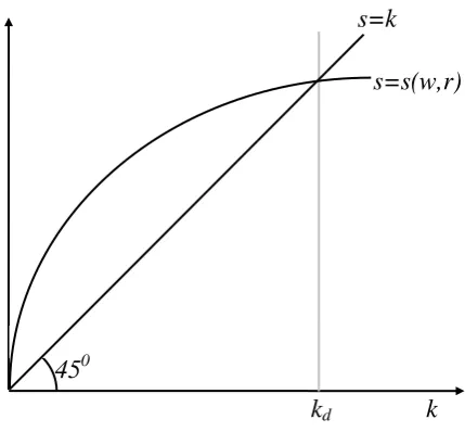
rate. The relationship between saving in equilibrium and the capital stock is illustrated in

Figure 3.1.

Figure 3.1: Saving and the capital stock

The positive difference between savings and the capital stock is the savings that go to buy

bubble assets. The bubble cannot be negative, so a capital stock of more than kd is impossible.

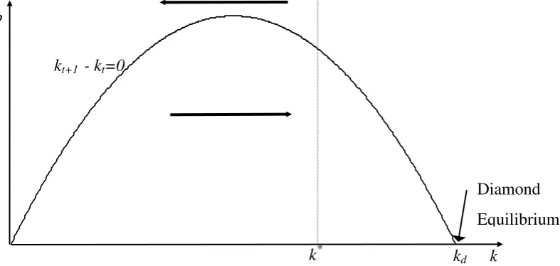
Figure 3.1 can be used to draw a figure of the bubble as a function of the capital stock, as in

Figure 3.2. In this figure the combinations of b and k that results in zero capital accumulation

are presented. Thus the depicted line gives the combinations of capital and the bubble when

kt+1=kt so that bs k k( , ) (1 n k) according to equ. ( 3.11b). As mentioned before, for a

bubble to exist, savings must be higher than investment for low levels of capital. Since the

7

Provided that u

 

k kd

s

s=k

s=s(w,r)

savings function is a decreasing function of capital, at some point the equilibrium level of

savings for a certain level of capital will be less for additional investment. Thus, the

kt1kt 0 curve is first upward sloping and then falling. At point kdthe bubble is zero. This is the Diamond equilibrium that the economy would reach if there were no bubbles. At this

point savings equals investment.

At any point above the kt+1-kt=0 line, the bubble takes up so much of savings that not enough

is invested. Production next period becomes less and investment is reduced more. The bubble

is too large for the economy to support it, and the capital stock decreases. The opposite is true

for any point below the line. The bubble is so small that the part of savings that goes to

investment will increase production next period so that investment will increase even more.

Savings will increase investment even in the presence of a bubble. The investment effect will

therefore increase capital below the kt+1-kt=0 locus, and reduce it above it.

Figure 3.2: Dynamics caused by saving in the bubble asset

3.5.2 The arbitrage effect

Differentiating the steady state solution of ( 3.11b) yields:

0



 



 

 

1 1

    

 



 



    

f s b n b f s b

n db b

f s b

n ds dkdk

, , ,

Which implies:

k

k* kd

kt+1 - kt=0

b

Diamond

 

 









 





 

 





bf s b ds

dk

f s b n n bf s b

bf s b ds

dk

bf s b

ds dk                  , , , , , 1

The second equality follows since we are in steady state so that f k( )n. By the assumptions made earlier, we have that db

dk ds dk

 0. So the steady state curve where

bt1 bt has a positive slope in Figure 3.3

8

. If we take the second derivative we get

d b dk d s dk 2 2 2 2 0

  if we use ( 3.14). Thus the b_t1 b_t locus has a positive slope, but at a

decreasing rate as in Figure 3.3. These properties can be explained as follows:

In steady state, when bt+1=bt, the arbitrage equation ( 3.11b) becomes

 





f s k k b

n n

,

1 . If

we start at the point where the capital stock is such that f k( )n and there is no bubble, and then increase the bubble, it takes up more of the savings, leaving less to be invested. The

marginal product (the interest rate) will therefore exceed the growth, if the capital stock is not

increased. So to keep f k( )n, k must increase. The steady state locus where bt+1-bt=0 is

therefore not vertical but upward sloping as mentioned earlier. The locus is increasing at a

decreasing rate with the capital k, because more capital is needed to facilitate a given increase

in the bubble if the arbitrage equation is to be in steady state ( f k( )n). The forces at the

right and the left hand side of the arbitrage steady state path is as follows

To the left the capital stock is so low that the marginal product exceeds the growth rate. The

economy is dynamically efficient. Arbitrage implies that the price per unit bubble must

increases at the same rate as the return on investments, f ( )k . For this to happen, we know

that the bubble in per capita terms must increase since the return on investment is higher than

the population growth. So, on the left hand side of the arbitrage steady state path when

 

f ( )k n the bubble, bt, must expand if the bubble asset is to give the same return as capital

relative to the growth.

8

To the right, the capital stock is so high that the growth rate exceeds the marginal product, the

economy is dynamically inefficient. Since the price per unit bubble must increase at a the same

rate as the interest rate, the bubble in per capita terms must decrease. So, on the right hand

side of the arbitrage steady state path when f ( )k n the bubble, bt, must contract if the

bubble asset is to give the same return as capital relative to the growth. This is illustrated in

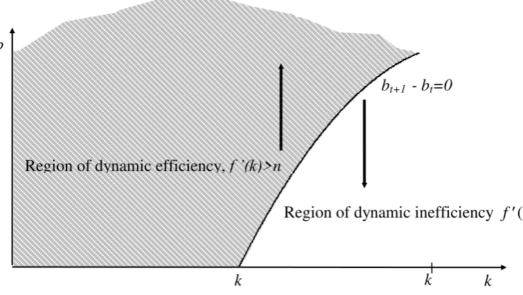
Figure 3.3

Figure 3.3: Dynamics caused by arbitrage

3.5.3 Dynamic efficiency and diamond equilibrium

For the bubble to converge to a stable equilibrium, the capital stock k* necessary for a non-bubble economy to be dynamically efficient, that is f(k*)n and b=0 , must lie between zero and kd. If not, the economy can never reach the point where the bubble will decrease (that

is where f k( )n), since there will be no forces under the k_t k_t1 locus that pull in the direction of no bubble. The bubble will increase forever and no equilibrium is possible.

To the right of k* we will have dynamic inefficiency, since f 

 

non bubble economy (the Diamond equilibrium at point kd) is dynamically inefficient, so

that f k( _d)n. This is a necessary condition for a general equilibrium to exist.

bt+1 - bt=0

b

k

Region of dynamic efficiency, f ’(k)>n

Region of dynamic inefficiency f ( )k n

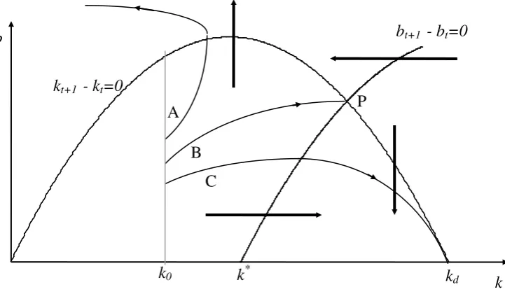
3.5.4 Trajectories

In Figure 3.4, I have drawn possible paths for a bubble starting at three different points, with

an initial capital stock at k0. The bubble starting at point B gives the path leading to the stable

equilibrium at P. The arbitrage effect and the investment effect affects the bubble just so much

that it will reach a general steady state (both effects are in a steady state).

Figure 3.4: The paths for different initial levels of the bubble

If the initial bubble is too large (e.g. point A), the arbitrage effect becomes very apparent, and

the investment effect becomes very small. Most of savings goes to buying bubble assets,

which will increase the capital stock too little to account for the strong arbitrage effect. Since

the capital stock does not increase as much as if the bubble had started in B, the interest rate

decreases and the bubble increases more. Eventually the bubble will cross the kt+1-kt=0 line,

and capital will decrease at an increasing rate at the same time as the bubble increase at an

accelerating rate. Finally this means that the capital stock becomes negative. Rational

behaviour does not allow such a path. People will know that this is not beneficial for them. It

is therefore not possible to be on a path above B and reach a general equilibrium, if people are

rational.

If the initial bubble is less than B (e.g. point C), it will converge to zero. The initial bubble

will increase less relative to investment than if it started at B or equivalently the arbitrage

effect will be small compared to the investment effect. This is because the smaller bubble

kt+1 - kt=0

bt+1 - bt=0

k0 k_d

A

B

C

P

b

results in higher capital accumulation, so that the interest rate decreases and consequently the

bubble increase less. At the point where growth is larger than the rate of interest, the bubble

(in per capita terms) will start to decrease if the bubble is to give the same return as

investment. The economy will therefore converge towards kd.

3.5.5 If the bubble asset paid dividends

In the theory described, the bubble asset was intrinsically useless. It was held because people

had confidence in that they could sell it later. Does this example apply if the bubble pays

dividends? The answer is yes. Since the bubble component of an asset must grow at the rate of

interest, and dividends are assumed to increase less than the interest rate, the present value of

the asset when it is discounted infinitely, will be the bubble component. The dividend in the

future will be negligible, but the bubble component will not.

The same argument rules out that a rational bubble can be negative. A negative bubble will

cause the price to become negative since the negative bubble must grow faster than the price.

Negative prices are not consistent with rational behaviour and consequently such bubbles in

this context are ruled out.

3.5.6 Bubbles, dynamic efficiency, Pareto efficiency and money

As we can see in Figure 3.4, a bubble can exist over time in a general equilibrium at P. A

bubble such as this will in fact be dynamically efficient and Pareto efficient, since it prevents

the economy from being in the inefficient competitive non-bubble Diamond equilibrium. It

can be argued that money is such a bubble. Money may be looked upon as an intrinsically

useless asset, which is only valued because people trust that it will be worth something in the

future to others.

Money may very well prevent the economy from ending in an inefficient state. In contrast to

the Diamond equilibrium where everything the economy saves is invested, money makes it

possible to save without investing. It therefore may reduce the capital stock and increases the

interest rate and thus make the economy efficient.

However this view may be more appropriate in relation to earlier times, when saving in

money do, such as lowering transactions costs which can be viewed as dividends, are more

important. Consumers and firms are therefore more likely to possess money as a

fundamentally priced asset. But money is held in large amounts by different investors through

out the world (private investors, banks and countries) as an asset. This money does not yield any significant transaction services, but is held to ensure a country’s local currency or as pure speculation.

Another, and possibly better example of rational bubbles, is gold. It yields no

services/dividends and its use is roughly limited to jewellery and electronic circuits. The

finding of new gold is also limited. The limited use of gold of course heightens its value, but

most of the known extracted gold resources are hidden in bank vaults, so at least a part of the

gold price can be said to be a rational bubble. This fits very well with the stable equilibrium

rational bubble. The bubble in «per capita terms» (the gold price adjusted for the economic

growth, which is the same as population growth, n, according to the OLG model) has been

rather constant in the past history, so that the actual gold price has increased at the rate of the

economy. Therefore, this may be a stable equilibrium. If everybody, countries and banks

included, suddenly found out that saving in gold was pointless, the price might drop to its

fundamental level. The price of gold would be equal to what the marginal buyer and seller

would be willing to pay for it to use it (since «production» of gold, which is the same as

exploring new mines whose sites have not yet been priced for its existence, is very limited). A

change in this stable equilibrium is in fact exactly what is happening at present. National

banks shifts their holdings from gold to bonds, causing the gold price to drop («The

Economist» no. 47, 1997).

3.5.7 Stochastic bubbles

We can now expand the model by introducing the probability that a bubble can burst. In this

stochastic model the bubble, bt, follows a process:

( 3.15) b

b

aq e

b e

t t

t

t t

 

 

 



1 1

1 1

probability q