A Comparative Study in Predicting Colon Rectum
Cancer using Auto Regressive Integrated Moving
Average (ARIMA) and
Artificial Neural Network (ANN) Models
S. Shenbaga Ezhil
Research Scholar Sathyabama University
Chennai 119
C. Vijayalakshmi
Asst. Prof., Dept. of Mathematics Sathyabama University
Chennai 119
ABSTRACT
Colon Rectum Cancer is one of the leading cause of cancer deaths worldwide. In this paper, a comparative study is made for the prediction of Colon Rectum Cancer using Auto Regressive Integrated Moving Average (ARIMA) and Artificial Neural Network (ANN). For more than twenty decades, Box Jenkin’s Auto Regressive Integrated Moving Average (ARIMA) technique is one of the most sophisticated extrapolation method for prediction. It predicts the values in a time series as a linear combination of its own past values, past errors and current and past values by using the concept of time Series. Artificial Neural Network (ANN) is a modern Non Linear Technique used for prediction that involve learning and pattern recognition. Based on the data the model is was modeled is designed by using two techniques for a period of 50 years (from 1960 to 2010) and the Mean Absolute Error (MAE), Mean Square Error (MSE), Mean Absolute Percentage Error (MAPE) and Root Mean Square Error(RMSE) are obtained to evaluate the accuracy of the models. Results show that ANN model perform much better than the traditional ARIMA model. Since early detection of cancer is the key to improve survival rate, prediction of Colon Rectum Cancer will greatly facilitate the doctors in the diagnosis of the disease.
Keywords
Auto Regressive Integrated Moving Average (ARIMA), Artificial Neural Network (ANN)
1.
INTRODUCTION
Cancer refers to cells that grow larger that 2mm in every 3 months and multiply uncontrollably and spread to other parts of the body. In this paper we have developed an Artificial Neural Network (ANN) model is developed for for Colon Rectum Cancer which can be used for all type of diagnosis and detection [1]. Artificial Neural Network systems are made to learn the cancer data by the use of training algorithms. Learning involves the extraction of rules or pattern from the historical data.
Since early detection of Colon Cancer is the key to improve survival rate, it is essential that doctors plan and provide proper therapy for each patient particularly when the risk factors of cancer are correctly determined. Also, the severity of the disease can be reduced to a great extent if it is detected early. Time, money expenses, hospital resources also can be effectively and efficiently managed. In general, Statistical Techniques like Kaplan-Meier and Cox Regression Analysis can be used for prediction. But these three method have
some some major drawbacks. ANN is thus an alternative approach in which they provide the prediction in an appropriate manner. Hence ANN is increasingly popular in recent analysis of cancer prediction.
2.
ARTIFICIAL NEURAL NETWORK IN
COLON
RECTUM
CANCER
PREDICTION
ANN is a branch of computational intelligence that employs a variety of optimization tools to learn from past experiences and use this prior training to predict and identify new patterns. In this neural network models have been used for the prediction of Colon Rectum Cancer.
ANN is a network that simulates our human brain functions. It is composed of parallel computing units called Neurons. These neurons can be connected in various ways to form different Neural Network architectures. The most popular architecture is the Multi-layer Perceptron (MLP). It consists of two or more layers of neuron in which the layers are connected in sequential manner. Each neuron in turn are connected to other neurons in the different layer by weighted path ways. Signals are sent through these pathways to the
Collect data set for Colon Rectum Cancer
Data processing
Simulate ANN models
Training and Testing phase
Prediction and Diagnosis Decision
[image:1.595.312.552.395.635.2]Performance Comparison of ANN models
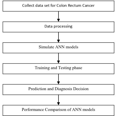
other neurons. Each neuron sums the weighted signals and transforms the resulting signal as the output of the neuron using an activation function. The output signal is then sent to the other neurons in the subsequent layers. The first layer of the network is called the input layer which receives signals from the data entering the network. The last layer is called the output layer which generates the outcome to the outside world. The overall complete methodology is shown in Figure 1.
3.
EXPERIMENTAL
RESULTS
OF
MULTI LAYER PERCEPTRON (MLP)
NEUTRAL NETWORK
The MLP uses the gradient descent to compute the new value of the weights and biases. It is quickly able to adjust the network weights giving a very good performance. The space denoted the error of the system for every combination of weights and biases is called as error space. The feed forward neural network architecture used in this experiment consists of two hidden layer along with one input and output layer respectively. The transfer function in hidden layer neurons and output layer neurons are hyperbolic tangent and identity. The performance function used was MSE.
3.1
Back Propagation Algorithm (BPA)
Back propagation Algorithm assumes that there is supervision of training of network. The method of adjusting weights is designed to minimize the sum of the squared errors for a given training data set. ANNs are developed by BPA in following steps.Step 1: Select an input and output variables and decide the architecture of ANN for modeling the variables.x presents the input , y hidden and z output layer.
Step 2: calculate the net inputs and outputs of the hidden layer neurons
Netjh =
1
1
N
i
wji x i ,yj =f(Net j h )Step 3: calculate the net inputs and outputs of the output layer neurons
Netk0 =
1
1
J
j
v kj yj ,zk =f(Netk0 )Step 4: update the weights in the output layer (for all k, j pairs)
v kj ← vkj +c λ (d k - z k )z k (1- z k)yj
Step 5: update the weights in the hidden layer (for all i, j pairs)
wji ← wji + c λ2 yj( 1 – yj )xi {
1
k
k
(dk -zk )zk ( 1 –z k )v kj }
Step 6: update the error term
E ← E + 1
k
k
(dk - zk )2and repeat from Step 1 until all input patterns have been presented (one iteration.)
Step 7: If E is below some predefined tolerance level (say 0.000001), then stop. Otherwise, reset E=0, and repeat from Step 1 for another iteration.
3.2
Predictors for the ANN
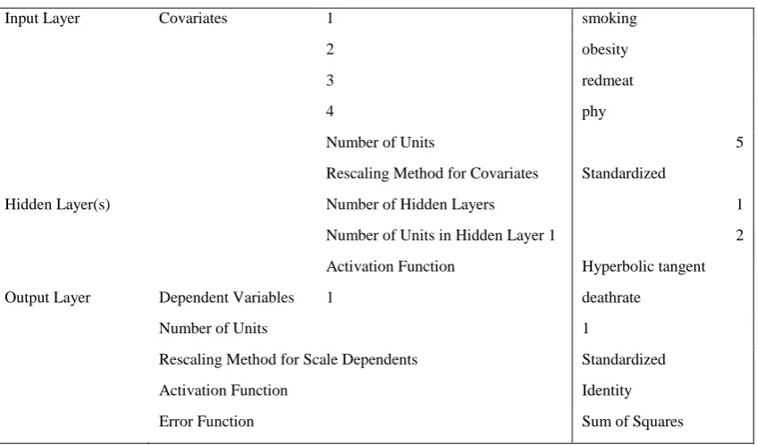
[image:2.595.88.512.494.743.2]There are five predictors for ANN which are smoking, obesity, red meat eating, physical activity and usage of aspirin and other medicines respectively. Mean Absolute Error (MAE), Mean Square Error (MSE), Mean Absolute Percentage Error (MAPE) and Root Mean Square Error(RMSE) were calculated for the output.
Table 1. Network Information
Input Layer Covariates 1 smoking
2 obesity
3 redmeat
4 phy
Number of Units 5
Rescaling Method for Covariates Standardized
Hidden Layer(s) Number of Hidden Layers 1
Number of Units in Hidden Layer 1 2
Activation Function Hyperbolic tangent
Output Layer Dependent Variables 1 deathrate
Number of Units 1
Rescaling Method for Scale Dependents Standardized
Activation Function Identity
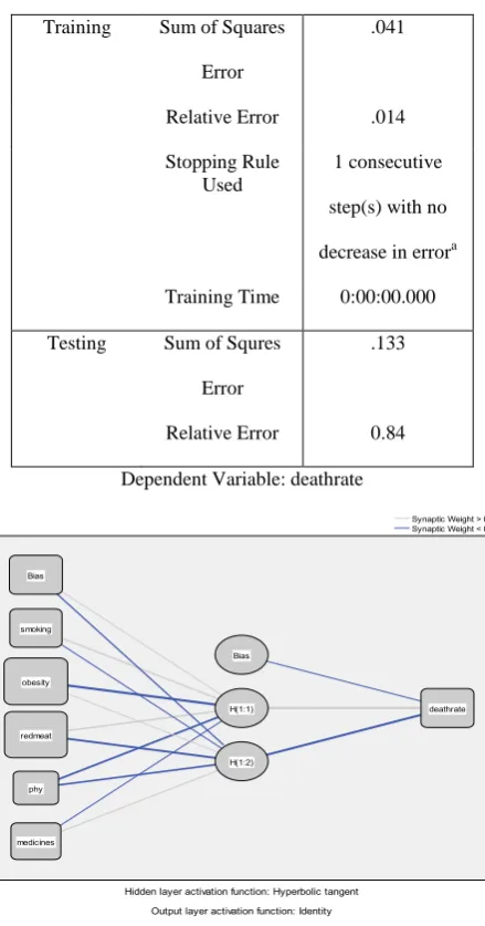
Table 2:Training and Testing Error of ANN
Training Sum of Squares
Error
.041
Relative Error .014
Stopping Rule Used
1 consecutive
step(s) with no
decrease in errora
Training Time 0:00:00.000
Testing Sum of Squres
Error
.133
Relative Error 0.84
[image:3.595.57.277.86.505.2]Dependent Variable: deathrate
Figure 2. ANN Network Diagram
Figure 3:Chart of predicted versus actual values
[image:3.595.334.522.286.424.2]Figure 4:Chart of predicted versus residuals
Table 3:Normalised Importance among the predictors
Importance Normalized Importance
smoking .159 46.4%
obesity .344 100.0%
redmeat .329 95.7%
phy .046 13.4%
medicines .122 35.4%
Simulation is carried out for various parameters and they were tested using many combination of parameters in independent experiments. The optimal prediction data for various ANN models were obtained by comparing with the parameter of error estimates such as Mean Absolute Error (MAE), Mean Square Error (MSE), Mean Absolute Percentage Error (MAPE) and Root Mean Square Error(RMSE).Among the predictors ,the most important factor influencing Colon Cancer is obesity,followed by eating red meat,smoking,taking medicines like aspirin and last of all lack of physical activity.
4.
FORECASTING
WITH
ARIMA
MODEL
Autoregressive Integrated Moving Average (ARIMA) is one of the popular linear models in time series forecasting during the past three decades popularized by George Box and Gwilym Jenkins in the early 1980s; as a result, ARIMA processes are sometimes known as Box-Jenkins models. ARIMA processes have been a popular method of forecasting because they have well-developed mathematical structure.
4.1
ARIMA Methodology
The art of ARIMA modeling involves the following steps:
The next step in the identification process is to find the initial values for the orders of parameters p, q. They could be obtained by looking for significant autocorrelations and partial autocorrelation coefficients. The Auto Correlation Function (ACF) and partial ACF (PACF) are very important for the definition of the internal structure of the analyzed series. Theoretically, both an AR (p) process and an MA(q) process should be associated with well-defined patterns of ACF and PACF.
(b) Estimation: At the identification stage, one or more models are tentatively chosen that seem to provide statistically adequate representation of the available data. Then we attempt to obtain precise estimates of the model by least squares as advocated by Box & Jenkins.
(c) Diagnostics: Different models can be obtained for various combinations of AR and MA individually and collectively. For the models obtained, perform diagnostic tests using
(1) Residual ACF (2) Box pierce Chi-square tests (d) Forecasting: ARIMA models are developed basically
[image:4.595.323.529.83.272.2]to forecast the corresponding variable.
Table 4: Model Description
Model Type
Model ID
Deathrate Model_1 ARIMA(0,1,0)
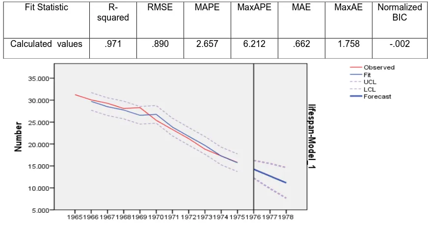
[image:4.595.78.514.350.580.2]Figure 5:Residual Chart of ARIMA ( 0,1,0)
Table 5: Model Fit of ARIMA (0,1,0)
Fit Statistic R-squared
RMSE MAPE MaxAPE MAE MaxAE Normalized BIC
Calculated values .971 .890 2.657 6.212 .662 1.758 -.002
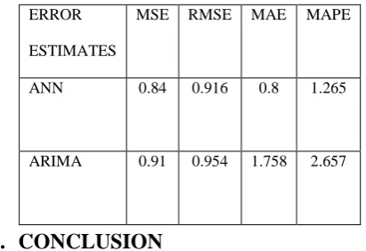
Table 6 :Error Estimates for ANN and ARIMA
ERROR
ESTIMATES
MSE RMSE MAE MAPE
ANN 0.84 0.916 0.8 1.265
ARIMA 0.91 0.954 1.758 2.657
5.
CONCLUSION
Data was modeled using ANN and ARIMA for a period of 50 years (from 1960 to 2010) obtained from SEER Cancer Statistics,USA.The Mean Absolute Error (MAE), Mean Square Error (MSE), Mean Absolute Percentage Error (MAPE) and Root Mean Square Error(RMSE) were calculated for the predicted values.
In this paper it can be seen that the prediction performance of ANN is better than the conventional statistical techniques such as ARIMA modeling. The above table shows that in all the error estimates ANN supercedes ARIMA modeling. It clearly indicates that linear relationship could not be assumed in this analysis. The non-linearity component of the relationship can be successfully dealt with using artificial neural network. This shows the effectiveness of ANN in the prediction of Colon Rectum Cancer.
6.
REFERENCES
[1] M.G. Kendall and A. Stuart, (1966), “The advanced theory of statistics”, Vol. 3. Design and Analysis and Time-Series, Charles Griffin & Co. Ltd., London, United Kingdom.
[2] G.E.P. Box and G.M. Jenkins (1970), “Time series analysis: Forecasting and control”, San Francisco: Holden-Day.
[3] C.W.J. Granger and P. Newbold, (1986), “Forecasting Economic Time Series” (Academic Press, San Diego).
[4] G.E.P. Box, G.M. Jenkins and G.C. Riesel, (1994), “Time Series: Analysis: Forecasting and control”, Pearson Education, Delhi.
[5] P.J. Brockwell and R.A. Davis, (1996), “Introduction to time series and forecasting” Springer.
[6] David B. Fogel, Eugene C. Wasson, Edward M. Boughton, Vincent W. Porto, and Peter J. Angeline, “Linear and Neural Models for Classifying Breast Masses”, IEEE transactions on medical imaging, vol. 17, no. 3, June 1998, pp 485488.
[7] Heng-Da Cheng, Yui Man Lui, and Rita I. Freimanis “A Novel Approach to Microcalcification Detection Using Fuzzy Logic Technique”, IEEE transactions on medical imaging, vol. 17, no. 3, June 1998, pp 442450.
[8] Ky Van Ha, “Hierarchical Radial Basis Function Networks”, 1998, EEE 1893 PP 18931898.
[9] S. Makridakis, S.C. Wheelwright and R.J. Hyndman, (1998), “Forecasting: methods and applications”, New York: John Wiley & Sons.
[10]Lubomir Hadjiiski, Berkman Sahiner, Heang-Ping Chan, Nicholas Petrick and Mark Helvie, “Classification of
Malignant and Benign Masses Based on Hybrid ART2LDA Approach”, IEEE transactions on medical imaging, vol. 18, no. 12, December 1999, pp 11781187.
[11]Taio C. S. Santos-Andrk and Anttinio C. Roque da Silva, “A Neural Network Made of a Kohonen’s SOM Coupled to a MLP Trained Via Backpropagation for the Diagnosis of Malignant Breast Cancer from Digital Mammograms”, 1999 , IEEE pp 36473650.
[12]Azra Alizad, Mostafa Fatemi, Member, Lester E. Wold and James F. Greenleaf, “Performance of Vibro-Acoustography in Detecting Microcalcifications in Excised Human Breast Tissue: A Study of 74 Tissue Samples” IEEE transactions on medical imaging, vol. 23, no. 3, March 2004, pp 307312.
[13]Kenneth Revett, Florin Gorunescu, Marina Gorunescu, Elia El-Darzi and Marius Ene, “A Breast Cancer Diagnosis System: A Combined Approach Using Rough Sets and Probabilistic Neural Networks”, EUROCON 2005, Serbia & Montenegro, Belgrade, November, 22-24, 2005, pp 11241127.
[14]Patricia Melin and Oscar Castillo: Hybrid Intelligent Systems for Pattern Recognition Using Soft Computing, StudFuzz 172, 85–107 (2005), Springer-Verlag Berlin Heidelberg.
[15]Xiangchun Xiong, Yangon Kim, Yuncheol Baek, Dae Wong Rhee, Soo-Hong Kim. “Analysis of Breast Cancer Using Data Mining & Statistical Techniques”, Proceedings of the Sixth International Conference on Software Engineering, Artificial Intelligence, Networking and Parallel/Distributed Computing and First ACIS International Workshop on Self-Assembling Wireless Networks (SNPD/SAWN’05) 2005 IEEE. [16]J.A. Cruz and D.S. Wishart, “Applications of machine
learning in cancer prediction and prognosis”, Cancer Informatics, Vol. 2, pp. 5978, 2006.
[17]Yuanjiao MA, Ziwu WANG, Jeffrey Lian LU, Gang WANG, Peng LI Tianxin MA, Yinfu XIE, Zhijie ZHENG “Extracting Microcalcification Clusters on Mammograms for Early Breast Cancer Detection” Proceedings of the 2006 IEEE International Conference on Information Acquisition August 20-23, 2006, Weihai, Shandong, China, pp 499504.
[18]T.Z. Tan, C. Quek, G.S. Ng a, E.Y.K. Ng, “A novel cognitive interpretation of breast cancer thermography with complementary learning fuzzy neural memory structure”, Expert Systems with Applications 33 (2007) 652–666.
[19]Al Mutaz M, Abdalla, Safaai Deris, Nazar Zaki and Doaa M. Ghoneim, “Breast Cancer Detection Based on Statistical Textural Features Classification”, 2008, IEEE, pp 728730.
[20]Anna N. Karahaliou, Ioannis S. Boniatis, Spyros G. Skiadopoulos, Filippos N. Sakellaropoulos, Nikolaos S. Arikidis, Eleni A. Likaki, George S. Panayiotakis, and Lena I. Costaridou, “Breast Cancer Diagnosis: Analyzing Texture of Tissue Surrounding Microcalcifications”, IEEE transactions on information technology in biomedicine, vol. 12, no. 6, November 2008 , pp 731738.
in breast cancer”, 4th IEEE International Conference on Intelligent Systems, 2008, pp 3843.
[22]Nuryanti Mohd Salleh, Harsa Amylia Mat Sakim and Nor Hayati Othman, “Neural Networks to Evaluate Morphological Features for Breast Cells Classification”, IJCSNS International Journal of Computer Science and Network Security, VOL. 8 No. 9, September 2008, pp 5158.
[23]Shakti K. Davis, Barry D. Van Veen, Susan C. Hagness and Frederick Kelcz, “Breast Tumor Characterization Based on Ultrawideband Microwave Backscatter”, IEEE transactions on biomedical engineering, vol. 55, no. 1, January 2008, pp 237246.
[24]Mohammad Sameti, Rabab Kreidieh Ward, Jacqueline Morgan-Parkes and Branko Palcic “Image Feature
Extraction in the Last Screening Mammograms Prior to Detection of Breast Cancer” IEEE journal of selected topics in signal processing, vol. 3, no. 1, February 2009, pp 4652.
[25]Shlomi Laufer and Boris Rubinsky, “Tissue Characterization with an Electrical Spectroscopy SVM Classifier”, IEEE transactions on biomedical engineering, vol. 56, no. 2, February 2009 pp 525528.