Assessing the Impact of Poverty Reduction Programs in Vietnam

Munich Personal RePEc Archive

Assessing the Impact of Poverty

Reduction Programs in Vietnam

Nguyen Viet, Cuong

1 December 2003

Online at

https://mpra.ub.uni-muenchen.de/25627/

1

Assessing the Impact of Poverty Reduction Programs

in Vietnam

Nguyen Viet Cuong1

Abstract

This paper aims to examine the poverty targeting and impacts of three poverty reeducation programs including programs ‘exemption of educational fees’, ‘provision with health care insurance’, and ‘micro-credit for the poor’ in Vietnam. It is found that the three programs have reached the poor quite well as compared to the international standard. The poor account for around 70 percent of participants in these programs. However the coverage of the programs over the poor is rather low, from 5 percent for the credit program to 11 percent for the health insurance program. There is no impact of the programs found on expenditure per capita, since it might take a long time for the programs to have large effects on income and expenditure. On average, households who were provided with preferential credit are more likely to have a pig, cow, buffalo, horse than other households.

Keywords: Poverty reduction program, impact evaluation, matching, household survey, Vietnam

JEL Classification: I38; H43; O11.

1

2

1. INTRODUCTION

Vietnam has set up poverty reduction as a major goal of development policy. The Government has implemented numerous programs to support the poor in all dimensionalities of living standards. Of which a major program that was launched in the year 1998 is the National Target Program on Hunger Elimination and Poverty Alleviation (HEPR Program).2 Its objective is to reduce the poverty and hunger in the period 1998-2000. In the year 2001 the HEPR Program was renewed for the period up to 2005 and merged with the Employment Creation Program to become now The National Target Program on Hunger Elimination and Poverty Reduction, and Job Creation. The program includes sub-programs targeted to the poor such as health care, education, and credit and some sub-programs supporting the poor communes.

A huge amount of finance is spent on the HEPR program. For two years 1999 and 2000, about 9600 billion VND from the State budget was put in the HEPR program. There is, however, little research on the impact evaluation of the poverty reduction programs in Vietnam. Most of evaluation reports simply describe the implementation and the output of the programs. Impact of a program on its participants should be measured by the change in welfare outcome of those participants that is attributed only to the program. Thus questions on the causal impact of the HEPR program on participants remain unanswered so far. The limitation can be explained partly by the data constraint. At least an ex-post single cross-section data on participants and non-participants in a program is required for impact assessment of the program.

Fortunately the Vietnam Household Living Standard Survey conducted by General Statistical Office of Vietnam in 2002 collected information not only on households’ characteristics but also on households’ participation in various poverty alleviation programs. Based on the survey data, impacts of three sub-programs of the overall HEPR are assessed in this research. These programs are: (i) the program of tuition exemption and reduction for the poor pupils; (ii) the program of provision of health care insurance for the poor; and (iii) the program of provision of credit for the poor households. These programs are aimed to improve the living standards of the poor through building human capital, i.e. education and health status, and asset capital, i.e. credit, and widely implemented throughout the country. Information on the impact assessment of the programs is very helpful for designation and modification of the HEPR programs.

For the estimation of program effects, the study will rely on the propensity score matching method to construct a comparison group of non-participants whose characteristics are similar to those of participants, and then simply compare outcomes between the treatment and comparison groups. For poverty targeting programs, there might be a large number of characteristics variables that affect both the program participation and outcomes. The standard method which can be used to solve the problem of endogeneity is instrumental variables regressions. However it is often difficult to find appropriate instrument variables that directly affect the program participation but not influence outcomes given the

2

3 participation. Although matching methods can be invalid in the case of “selection based on unobservables”, it is robust to the bias due to “selection based on observables”. In addition, econometrics models have to invoke assumptions on functional relationship between the outcomes, treatment variables, and the explanatory variables, while the propensity score matching does not.

The paper is organized into 5 sections. The second section describes the HEPR programs, and three sub-programs to be assessed. Section 3 presents the methodology of impact assessment used in the study. Then section 4 reports the empirical results of the impact assessment of the three programs. Finally some conclusions are drawn in section 5.

2. PROGRAMS OF HUNGER ELIMINATION AND POVERTY REDUCTION

2.1. Overview of Poverty Alleviation Programs

Poverty rate declined dramatically in Vietnam during the period 1990s. Between 1993 and 1998, the proportion of people with per capita expenditures under the poverty line dropped sharply from 58 to 37 percent. The rate of poverty reduction, however, is lower in recent years. There is a decline of only 8 percentage points in poverty rate from 1998 to 2002 (World Bank, 2003).

To reduce poverty the Government has implemented many poverty reduction programs and projects affecting all facets of the people’s living standards. There are two major programs of hunger eradication and poverty reduction, which consist of different component projects.

The first is the national target program on hunger elimination and poverty reduction (HEPR) that was launched by the Government in 1998, aiming at eliminating hunger and reducing poverty in the period 1998-2000. The Ministry of Labor, War Invalids and Social Affairs (MOLISA) is assigned to execute the program. The program includes the following projects targeted at the poor and poor communes:3

- Investment project on infrastructure construction (excluding the rural clean water supply) and population rearrangement.

- Project on support of production and the development of branches and crafts. - Project on support of credits for the poor.

- Project on support of education for the poor. - Project on support of health care for the poor.

3

4 - Project on guidance for the poor to earn their living and promote agricultural, forestry

and fishery production.

- Project to raise qualifications of the contingent of cadres engaged in the hunger elimination and poverty alleviation work and cadres in poor communes.

- Projects on sedentarization, migration and new economic zones. - Project in support of ethnic minority people facing fierce difficulties.

In the year 2001 the Program 133 was renewed (for the period up to 2005) and merged with the Employment Creation Program to become now the national target program on HEPRJC (Hunger Elimination and Poverty Reduction, and Job Creation). The employment creation program has been put into operation since 1998, aiming at reducing the unemployment rate in the urban areas, and increasing the working time in the rural areas, rearranging the employment structure appropriate for the economics structure for the sake of the people’s living standards.

The second program - the Program 135 – with the standing body organization of the Committee for Ethnic Minorities and Mountainous - Areas was launched at almost the same time to improve the living standard of the poor in mountainous and remote communes with special difficulties. The focus of the program is place on the construction of infrastructure such as the communication system, the drinking water and power-supply systems. Other components of the programs include projects on agricultural and forestry development, and projects on development of human resources for mountainous and rural communes and villages.4

At the end of the year 2000, the Government decided to consolidate some components projects of the Program 133, e.g. infrastructure construction project, and project on training cadres under the Program 135 to enhance the effectiveness of investments in communes with special difficulties.

2.2. Poverty Alleviation Programs to be Assessed

The assessment of poverty targeting in the research relies on the data from the Vietnam Household Living Standard Survey conducted by the General Statistical Office of Vietnam in 2002. The survey covers 29600 households located in about 2960 communes. The survey collects of some information on the participation of households and communes into various poverty alleviation programs/projects. The features of the survey will be described in more detailed in section 4.1 “Data Source”.

5 selected for impact evaluation. Firstly these programs are aimed to improve the living standards of the poor through building human capital, i.e. education and health status, and asset capital, i.e. credit. Secondly these programs are widely implemented throughout the country, allowing a relatively large number of observations that are covered by the programs in the survey. Thirdly the survey collects information on the participation on households in the programs, and welfare indicators that can be considered as direct outcomes of the program, e.g. the schooling ratio, educational expenditure, or fees and times of health care treatment.

Program of Tuition Exemption and Reduction for the Poor Pupils

Since the year 1998 the Government has implemented the program of education assistance for the poor children and ethnic minority children living in the communities with special difficulties. The program of education assistance is a component of the HEPR program, and has been designed to cover two phrases: the first lasted from 1998 to 2000, and the second is from 2001 to 2005. For the period 1998-2000 the program has set several specific objectives. The first is to eliminate the illiteracy and the dropping out of the school. The second is to create conditions favorable for the poor children to improve their educational degrees. Finally the program aims to reduce the disparity in living standards between the poor and non-poor children. The program of education assistance has several components consisting of exemption and reduction of educational contribution and tuition for pupils, provision of books and notebooks, scholarship for ultra-poor pupils and students, and provision of materials for schools of ethnic minorities. Of which the component program of exemption and reduction of educational contribution and tuition has the widest effects in aspects of the number of beneficiaries and the amount of allocated funds. It should be noted that the primary pupils do not have to pay tuition fees, but still have to make payments for educational contribution to their schools. The primary pupils that participate in the program benefit from exemption and reduction of educational contribution.

The program of education assistance is slightly modified in the second period 2001-2005. In addition to the program components as the first period, the program also provides the material support for schools of ethnic minority pupils.

Program of Provision of Health Care Insurance for the Poor

The program “Health support for the poor” aims to provide the poor with the access to high-quality health care services. It includes three main components: (i) provision of the health care card for the poor; (ii) exemption and education of health care fees for the poor; (iii) provision of medicines, health facilities, and human resources for health centers in localities.

4

6 The sub-program “Provision of the health care card for the poor” has been implemented since the year 1999. The target group of the program is the very poor persons who cannot afford the health treatment. It should be noted that this program is implemented in two ways. The first is to provide the poor with health insurance cards. The second is to provide the poor the free health care certificates. When holding a health care card the poor can get exemption and reduction of health care fees in State health center.

Besides, the poor can also get exemption or reduction of health care fees when showing the poor household certificate. This certificate is provided for poor households by the commune authorities based on MOLISA’s criteria.

Program of Provision of Credit for the Poor Households

The program has the objective to increase the income for the poor who have the incentive to develop production but lack the capital. To get the access to credit the households have to meet the following criteria:

- Being classified as the poor households by the commune authorities according to the classification criteria of MOLISA.

- Having the working capacity.

- Using the loan for the purpose of production.

The average loan is equal to from 2.5 to 3.5 million VND a household. The loan should not be larger than 7 million VND. There is no mortgage required. The credit should be returned after a circle of production (thereby depending on sort of production). The middle-term credit will be returned after 3-5 years.

3. IMPACT ASSESSMENT METHODOLOGY

3.1. Methodology of Propensity Score Matching

The main objective of impact evaluation of a program is to assess the extent to which the program has changed outcomes of program participants. In other words impact of the program on the participants is measured by the change in welfare outcome that is attributed only to the program. To make the definition more explicit, suppose that there is a program assigned to individuals i’s in population P. Let denote Ti as a binary variable of participation

in the program of individual i, i.e. Ti equals 1 (or 0) if individual i participates (or not

7 variable when individual i does not participate in the program. The expected impact of the program on the outcome of the participants is measured as follows:

) 1 T Y ( E ) 1 T Y (

E _{i1 i} = − _{i0 i} = =

τ . (1)

The program impact is equal to the difference between the average outcome when the participants did participate in the program and the average outcome of the same participants when they had not participated in the program. In evaluation literature τ is sometimes called the average treatment effect on treated.

The fundamental problem in measuring the program impact is that the outcome of the participants if they had not participated, i.e. Y_i0T_i =1 cannot be observed. This is counterfactual to be estimated. If the program is assigned randomly to individuals in the population, the potential outcomes Y_i0 ,Y_i1 are independent of the program assignment, denoted as: Y_i0 ,Y_i1 ⊥T_i. The outcome of non-participants E(Y_ioT_i =0)can be used to estimate E(Y_i0T_i =1), and the program impact on the participants is measured simply by the difference in the mean outcomes between the participants and non-participants in the program: ) 0 T Y ( E ) 1 T Y ( E ) 1 T Y ( E ) 1 T Y (

E _{i1 i} = − _{i0 i} = = _{i1 i} = − _{i0 i} = =

τ . (2)

It should be noted that a so-called stable unit treatment value assumption is always assumed in literature of program impact evaluation. This assumption states that outcomes of individual i do not depend on the participation in the program of other individuals. In other words the program has no spillovers or general equilibrium effects. Obviously if there is spillover effect, the outcome E(Y_i0T_i =0) cannot restore the counterfactual outcome of participants in absence of the program since it is also contaminated by the program.

If the program is aimed to reduce poverty, it is often designed to target the poor. Participants are selected into the program not randomly but based on several criteria such as levels of income, or expenditure, and geographical location. The condition Y_i0 ,Y_i1⊥T_i is no longer holding. The participants and non-participants are systematically different in some characteristics, and will respond in different way to the program. The expected outcome of non-participants, E(Y_i0T_i =0) is not equal to the expected outcome of the participants if they had not participated in the program, E(Y_i0T_i =1).

In order to identify the program impact Rubin (1977) proposed an assumption called conditional independence assumption. This assumption states that given a set of variables X the potential outcomes Y_i0 ,Y_i1 are independent of the program assignment:

i i 1 i 0

i ,Y T X

Y ⊥ . (3)

8 counterfactual non-participation outcome of the participants after conditioning on the variable set X: ) 0 T , X Y ( E ) 1 T , X Y ( E ) 1 T , X Y ( E ) 1 T , X Y ( E ) 1 T Y ( E ) 1 T Y ( E i i 0 i i i 1 i i i 0 i i i 1 i i 0 i i 1 i = − = = = − = = = − = = τ

. (4)

Thus, if the set of variables X can be observed, a comparison group (also called control group) is constructed so that their characteristics are similar to those of the participants in program (called the treatment group). The difference between the treatment and comparison groups is that the treatment group participated in the programs while the comparison group did not. If such a comparison group is found, the program effect on the participants can be calculated simply as the average difference in outcomes between the treatment and comparison group.

For a comparison group to be found, it is assumed that there exists a so-called common support region over the participants and non-participants. It means that there are still individuals who do not participate in the program but have characteristics similar to those of participants.

The comparison group is constructed by matching each participant with non-participant based on the similar variables X. This matching method, however, is very difficult to implement. As the number of characteristics used in matching increases, the chances of finding a match to a participant are reduced. When the characteristics contain continuous variables it is almost impossible to find an identical match. Even if a match is found based on approximate value of characteristics it is unclear how these characteristics should be weighted.

Fortunately the multidimensionality problem of matching is solved by the Rosenbaum and Rubin (1983). They show that if the outcomes Y_i0,Y_i1 are independent of the program assignment given by the set of variables X, then they are also independent of the program assignment given the probability of being assigned to the program p(Xi) (called

propensity score): ) X ( p T ) Y , Y ( X T ) Y , Y

( _{i0 i1} ⊥ _{i i i0 i1} ⊥ _{i i} . (5)

The program effect on the participants can be estimated conditioning on the propensity scores: ) 0 T ), X ( p Y ( E ) 1 T ), X ( p Y (

E _{i1 i i} = − _{i0 i i} = =

τ . (6)

3.2. Estimation of Propensity Score and Program Impact

non-9 participant based on the closeness of propensity score. The second is to compute the program impact using values of outcome of the treatment and comparison groups.

The construction of the comparison group is started with the prediction of the propensity score by the logit model. The probability of being selected into program can be expressed as a logit function of covariates X:

(

)

i F X

P = α+β , (7)

where P is the probability of being selected into the program of individual i , i Pi=1for

participants, and P_i=0 for non-participants. X_i is a set of characteristics variables.

Ideally all variables that are expected to affect the program participation and outcome should be included in the logit regression. It is meant that all information on assignment mechanism of the program need to be observable. It is worth noting that in case of ex-post assessment using single cross section data, the explanatory variables are required not to be contaminated by the program process.

Once the propensity scores, Pˆ are predicted for all individuals, the comparison _i group can be constructed by matching participants with non-participants based on their propensity scores. Each participant can be matched with one or several non-participants depending on schemes of estimation of program impact. This research examines two ways to establish the comparison group. In the first way each participant is matched with its nearest neighbor participant. The nearest neighbor to participant i is defined as the non-participant j that has the closest value of the propensity score. In other words the nearest match is found by minimizing the absolute value of

(

)

non-participants. In the second way the comparison group is constructed by matching each participant with three nearest neighbor non-participants.

10 should be balanced in all strata.5 If there exists a covariate not balanced in many strata, e.g. three strata, the comparison group should be reconstructed by modifying the logit model of propensity score. Variables that are considered as less important in determining the program participation and outcomes can be dropped from the model. Another way is to add some interaction terms or higher-order terms of characteristics variables.

After a comparison group that has characteristics covariates similar to those of the treatment group is constructed, the average program effect on the treatment group is estimated as follows:

= ∈

− =

τ

N

1

i jM

0 j 1

i

j

Y M

1 Y N

1

ˆ (8)

where Y is the post-program outcome of matched participant i , i1 Y is the outcome of non-j0

participant j that is matched to the participant i . N is the total number of matched participants. M_j is the set of non-participants s'j that are matched to participant i , and M is the number of non-participants in a set. In the research the value of M equals 1 or 3, depending on the comparison group is constructed by the nearest neighbor matching or three-nearest-neighbors matching.6

4. EMPIRICAL RESULTS

4.1. Data Source

The analysis of the research relies on the data from Vietnam Living Standard Survey (VHLSS) conducted in the year 2002. The 2002 VHLSS is conducted by the General Statistical Office of Vietnam (GSO). The survey collects information through household and community level questionnaires. At the household level information collected can be divided into 9 sections including basic demography, employment and labor force participation, education, health, income, expenditure, housing, fixed assets and durable goods, the participation of households in the most important poverty programs. The commune questionnaires collect information on commune characteristics that affect the living standards of the people in communes. The commune questionnaires is organized into 8 sections consisting of demography and general situation of commune, general economic condition and

5

The method of testing the equality in mean of covariates within stratum is proposed by Dehejia and Wahba (2002). They perform the test for all the participants and non-participants after estimating the propensity score. In this research the test is applied for the treatment and comparison groups after they are matched. Since what we need is the similarity of covariates between the treatment and comparison groups.

6

11 aid programs, non-farm employment, agriculture production, local infrastructure and transportation, education, health, and social affairs.

The full household sample of the 2002 VHLSS covers the 75000 households. This sample is divided into two sub-samples: one sample with 30000 households and another with 45000 households. The difference between these two samples is that the sample of 30000 households collected detailed information on consumption expenditure, while the sample of 45000 households did not.

At the time of the research being conducted, the micro-data of sample of 30000 households has been processed and released to users. The basic sample frame of this sample is obtained from the Population Census conducted in the year 1999. The selection of the sample of 30000 households follows a method of stratified random cluster sampling so that it is representative for national, rural and urban, and regional levels. The sample is divided further into 4 sub-samples. Each one covers 7500 households and is conducted in a quarter in 2002 in order to eliminate information bias due to seasonal effects. However after processed and cleaned the number of households in the sample is reduced to 29518.

Information on commune characteristics is collected from 2960 communes. Commune data can be linked with household data to assess relationship between characteristics of households and characteristics of communes in which the households are located.

4.2. Poverty Targeting of HEPR Programs

The household questionnaires collect information on the participation of households in three poverty alleviation programs that are evaluated in the research. A household is regarded as a participant (beneficiary) in the program “Tuition exemption and reduction for the poor pupils” if the household has at least a child who has attended primary or secondary school and received the exemption and reduction of tuition and contribution due to poor or ethnicity status in the past 12 months before the point of interview time.7 A household is considered as a participant in the program “Provision of health care insurance for the poor” if at least a member of the household has been provided with a health care card during the past 12 months before the time of interview. For the program “Provision of Credit for the Poor Households”, a household is regarded as a participant if the household has been provided with loan from the Bank for the Poor during the past 12 months before the time of interview. Table A.1 in Appendix describes the definition of participants in the three HEPR programs based on the 2002 VHLSS questionnaires.

Table 1 presents some statistics to assess how well the three programs reach the poor and non-poor households. The second column shows the percentage rate of beneficiary

7

12 households to all households. Column from 3 through 5 give percentage rates of beneficiary households who are classified as the non-poor, the poor and food poor. The percentage rate of beneficiaries who are found non-poor is also called the leakage rate. The last two columns present the percentage rates of the participating households among the poor and the food poor households. This is also called the coverage rate of the programs over the poor and food poor households. A good poverty targeting will have a low leakage rate and a high coverage rate.

Table 1: The coverage and leakage percentage rates of the programs

Program Percent of

households with/who

Percent of beneficiary households who are

Percent of beneficiary households

Non-poor Poor Food

poor

Among the poor households

Among the food poor households

(1) (2) (3) (4) (5) (6) (7)

Exemption for

education fees 4.3 32.9 67.1 35.5 11.3 16.9

Health care

card 3.9 33.3 66.7 37.3 10.2 16.1

Access to

subsidized credit 1.9 28.6 71.4 34.7 5.3 7.2

Source: Estimated from VHLSS 2002

In the research the food poor are defined as those who have the per capita expenditure a year lower than the food poverty line. This food poverty line is set up by the GSO at 1383 thousand VND (equivalent to USD 89) which allows for consumption of 2100 calories a day, but with no allowance for essential non-food expenditures.8 Thus any non-food expenditure made by households on or below this poverty line is at the expense of an adequate nutritional intake. The overall poverty line that is referred to most frequently in government statistics and international comparison has an allowance for essential non-food consumption such as clothing and housing. Households lower than the overall poverty line are considered as the poor. This poverty line is equal to 1917 thousand VND (approximately USD 124) for the year 2002. The poverty lines in Vietnam have been calculated to take account of regional price differences and monthly price changes over the survey period.

It is shown that the poor account for around 70 percent of participants in these programs. In other words, the leakage rate of these programs is about 30 percent. These leakage rates are not high by international standards (Coady et. al., 2002). However the coverage of the programs over the poor and the food poor is quite low. The percentage rates of the poor households having access to the programs “Exemption of educational fees” and “Provided with health care insurance” are 10.2 and 11.3 percent, respectively. For the program “Credit for the poor” only 5.3 percent of the poor households participate in the program. The coverage rates over the food poor households are slightly higher since the number of the poor households is larger than the number of the food poor households.

The distribution of the beneficiaries across the expenditure quintiles of all households is also examined to see whether or not a program is progressively pro-poor. This

8

13 progressiveness of the programs is presented in Table 2. The distribution pattern of beneficiaries is quite similar for three programs. The poorest quintile accounts for largest share of about recipients, about 55 percent, while the richest quintile has the recipient share of under 5 percent.

Table 2: Distribution of Beneficiary Households by Quintiles

Programs Distribution of beneficiary households by quintile

Poorest Near-

Poorest

Middle

Near-Richest

Richest Exemption for

education fees 53.1 25.0 12.7 6.9 2.4

Health care card 52.3 21.7 16.1 5.2 4.7

Access to subsidized

credit 56.3 21.9 14.7 5.4 1.7

Source: Estimated from VHLSS 2002

An alternative way to examine the pro-poor progressiveness is to use a so-called concentration curve that portrays the cumulative proportion of beneficiary population versus the cumulative proportion of population ranked by expenditure per capita. If the horizontal axis represents the cumulative proportion of all households ranked by expenditure per capita, and the vertical axis represents the cumulative proportion of participating households, the further the concentration curve is above from the diagonal (45-degree) line, the better the program targets the poor households. The figure of concentration curve gives visible comparison of poverty targeting of the HEPR programs.

Figure 1 presents the concentration curve for the three HEPR programs. The long-dash line shows distribution of the poor households over all households ranked by expenditure per capita. If the concentration curve of a program lies above this the long-dash line, all participants in the program are the poor. Then the poverty targeting is perfect with the leakage rate of zero. It is shown that the three programs have similar distribution of participants over the poor households.

Figure 1: Concentration curve of program

Concentration Curve: Program “Exemption for Education Fees”

Concentration Curve: Program “Health Care Card” C u m u la ti v e p e rc e n ta g e o f p a rt ic ip a ti n g h o u s e h o ld s

Cumulative percentage of households ranked by expenditure per capita

0 20 40 60 80 100

0 20 40 60 80 100 C u m u la ti v e p e rc e n ta g e o f ta rg e te d p o p u la ti o n

Cumulative percentage of households ranked by expenditure per capita

0 20 40 60 80 100

14 Concentration Curve: Program “Access to

Subsidized Credit”

C

u

m

u

la

ti

v

e

p

e

rc

e

n

ta

g

e

o

f

ta

rg

e

te

d

p

o

p

u

la

ti

o

n

Cumulative percentage of households ranked by expenditure per capita

0 20 40 60 80 100

0 20 40 60 80 100

Source: Estimated from the 2002 VHLSS.

4.3. Impact of HEPR Programs

Estimation of Propensity Score

The first step in the impact assessment is to predict the probability of participating in a HEPR program of all households using a logit model. The dependent variable is a binary one which takes 1 if household i participates in a HEPR program, and 0 if household i does not. The main problem in the estimation is how to select explanatory variables. As mentioned above all variables that are exogenous to the program assignment and expected to affect the program assignment as well as outcomes should be included in the logit regression.

Outcome variables selected in this research include the direct and indirect outcomes. For all three programs indirect outcome is expenditure per capita which can be considered as a general indicator of living standards. However measuring the impact of HEPR programs using expenditure per capita as outcome is confronted with several difficulties. Firstly the programs are assessed after less than one year of implementation, since the survey asks households if they have participated in the programs in the past 12 months. Within such a short time the programs “Reduction for education fees”, “Health care insurance card”, and “Credit for the poor” cannot have significant impact on the income generating capacity, and thereby expenditure of households. Secondly there are many other programs targeted at the poor that are operating at the same with these three programs. Other contemporaneous programs might have effect on expenditures of both treatment and comparison groups, making it very difficult to capture truly impact of the programs in question.

15 of the program “Reduction for education fees”.9 In addition using direct outcomes to measure impact of the three HEPR programs also ensures the validity of assumption “Stable unit treatment value”, since they are hard to be contaminated by the participation of other households.10 Direct outcomes that are used in the research are described in Table A.2 in Appendix.

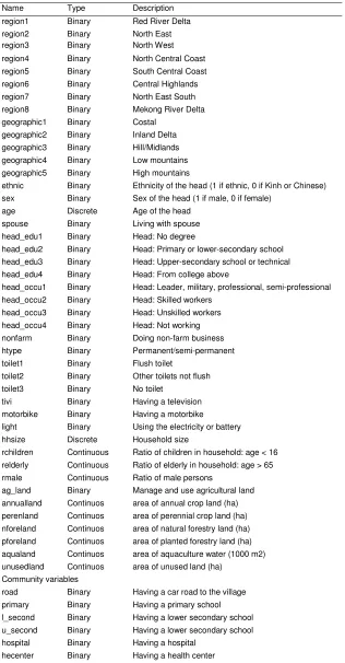
The VHLSS 2002 collects detailed information on household characteristics, allowing for a relatively large number of explanatory variables. The richness of data set is expected to ensure that information on program assignment can be observed, and the assumption of conditional independence would hold. The number of the explanatory variables is 50. These explanatory variables can be divided into three categories: (i) geographic location including the dummy variables of regions and geographic type of areas where households are located; (ii) household characteristics including household composition, asset ownership, characteristics of household head such as age, gender, ethnicity, education and occupation; (iii) commune characteristics including dummy variables of road, schools, and health centers. Appendix 1 describes the explanatory variables used in the estimation of probability of being selected into a HEPR program.

The logit regression is applied separately for urban and rural areas. This is because the model for the whole sample with a dummy variable of urban area gives some estimated coefficients with unexpected sign. In addition separate models for urban and rural areas also produce higher values of R-squared. The results of the logit regression for three HEPR programs are presented in Tables in Appendix.

It should be noted that the ultimate purpose of the propensity score is to balance covariates between the treatment and comparison groups. If there are many covariates that are not balanced after the matching, the estimation model of propensity score should be revised. The models reported in Appendices from 2 to 7 are obtained after several modifications so that the predicted propensity score can be used to produce a good comparison group. Once the balance of covariates is achieved, there is no concern about the problems of goodness of fit.

Matching and Assessment of Comparison Group

The comparison group is constructed in two ways: one nearest neighbor and three-nearest-neighbors matching. To ensure the quality, the research applies bounds to the matches, i.e. the matches are only accepted if the absolute value of difference in propensity score between the participants and matched non-participants,

(

)

9

Thus direct outcomes of a program are not affected by other programs, e.g. it is hard to say the program “Health care insurance” has significant effect on the schooling rate of children.

10

16 In addition the matching is performed within sub-groups: urban/rural areas, regions, ethnicity, and MOLISA’s classification of poor households. This matching strategy attaches more importance to the four variables. A participant and its corresponding matched non-participants are located in the same urban (or rural) area, and region, and belong to the same group of ethnicity, and poor households classified by MOLISA. In Vietnam the variables urban/rural areas, regions, and ethnicity are correlated strongly with the socioeconomic and cultural characteristics of households, thereby the outcomes of households. The commune authority’s classification of poor households based on MILISA criteria is one of important conditions that a household should meet in order to get access to a HEPR program.11 In other words the variable “Classification of poor household” has strong effect on the probability of being selected in each of three HEPR programs. However this variable should not be added to the logit regression, since it is strongly correlated with other explanatory variables. This problem can be avoided by the matching on this variable.

It should be noted that the matching of participants in the program “Health care card” is performed in a different way as compared with the other two programs. As mentioned in section 2.2 the program “Health care card” is one component of the overall program “Health support for the poor”. Households who are provided with a poor household certificate can also get exemption or reduction of health care fees when using health treatment. This fact can make the comparison contaminated. One way to solve this problem is to drop households with a poor certificate in the non-participant sample before matching implementation, but the survey does not collect information on whether a house is holding a poor certificate. An alternative way is to drop all households who are classified as poor households. Because before receiving a new poor certificate, a household needs to be classified as a poor household. However since a poor certificate is updated every two years, there can be households who were provided an old poor certificate before the time of being classified as the poor. Although this dropping cannot ensure that there is no household in non-participants sample holding a poor certificate, it is still the best way given the available data.

The dropping of these households does not violate the condition of common support region. The percentage of households being classified as poor over all households is 11.1 percent, while the percentage of households who are actually found poor is 25.6 percent. There still exist households with similar characteristics as the participants not participating in the program. This solution, however, can reduce the quality of matching, since the best matches might be dropped.

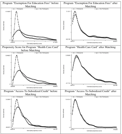
The number of participants and non-participants that are matched by the method of one-nearest-neighbor matching is presented in Appendix 8, 9 and 10 for three HEPR programs.12 Figure A.1 in Appendix graphs the kernel density of estimated propensity score

11

The commune authority classifies poor households based on the poverty line of MOLISA Using this poverty line, a household in mountainous and island areas is classified as poor if their monthly income per capita is lower than VND 80 000. In plain land rural areas, poor households are those with monthly income of below VND100 000, and in urban areas, those with monthly income of below VND150 000. Besides other basic need indictors such as health status, education, and household assets can also be considered in the process of classifying poor households.

12

17 of participants and non-participants before and after construction of comparison groups. It is shown that the treatment and comparison group have very similar distribution of propensity scores for all three programs. The quality of matching is assessed by the test for equality of covariate mean. Appendix from 11 to 13 give the mean value of covariates, and the P-value to reject the hypothesis of equality of covariate means between the treatment and comparison groups. For the program “Exemption for education fees”, there is only one covariate for which the hypothesis of mean equality can be rejected at significant level of 0.01. The number of covariates that are not balanced under the similar mean-test for the programs “Health care card” and “Access to subsidized credit” is 0 and 4, respectively. When the mean-test are examined within each of ten blocks, only a small number of covariates that are not balanced in some blocks (see Appendix).

Impacts of the HEPR Programs

Table 3, 4, and 5 present the estimated effect of each program on the participants. In these tables, the second and third columns present the mean of outcomes for treatment and comparison groups. The fourth column gives the estimated impact of a program measured by the difference in outcome means between treatment and control group. To calculate standard errors of the estimated impact the research uses the usual method of bootstraps with 100 replications.13 The last two columns present the 95% confidence interval of the estimated impact.

Table 3: Estimated Impact of Program “Exemption for Education Fees”

Outcomes Treated Matched Difference Std. Error 95% Conf. Interval

One-nearest-neighbor matching

Schooling rate 81.22 66.39 14.83 2.24 10.39 19.26

Education expenditure 193.65 247.27 -53.63 15.39 -84.16 -23.10

Expenditure per capita 1794.50 1808.76 -14.26 49.17 -111.81 83.30

Three-nearest-neighbors matching

Schooling rate 81.22 70.03 11.18 2.20 6.82 15.55

Education expenditure 193.65 246.64 -53.00 12.82 -78.43 -27.57

Expenditure per capita 1794.50 1841.17 -46.67 43.27 -132.52 39.18

Note: For definition of measurement unit, see Table 4

Source: Estimated from the 2002 VHLSS.

Table 3 shows that the program “Exemption for education fees” has statistically significant effect on the schooling rate. According to the one-nearest-neighbor matching, the average schooling rate of the treatment group is 11 percentage points higher than that of the comparison group. The program also helps the participants reduce the education expenditure. The average education expenditure per pupil of the treatment group is statistically lower than that of the comparison group. However the program does not has statistically significant impact on consumption expenditure per capita. Education is expected to have long-term

13

18 effect. When children become mature their educational knowledge will improve their earning capacity, and the living standards will be better-off in the long-term. The method of three-nearest-neighbors matching also produces a similar trend in impact estimation.

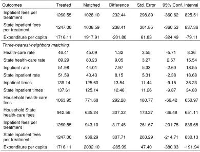
Table 4 presents the estimated impact of program “Health care card”. On average households with a health care card are more likely to use the healthcare services. It is a pity that the survey does not collect information on how many times a person uses the health services. It is found that the treatment group has higher spending on the health treatment than the comparison group. This could be a result from a higher times of using the health services. However all these differences in health care outcomes are not statistically significant at 5% level.

A reason why the impact of the program is limited might be the low level of health care card value, sometimes set as low as 30,000 VND. Depending on kinds of health care cards, the holders can get different level of fee reduction. This reduction is negligible amount compared to the non-treatment costs the poor have to incur, such as traveling costs and medicine. Thus the program is not much successful in stimulating the poor households to go the health center. They only use the health treatment when facing serious health problems. In these cases even if they do not have a health care card, they do have to come health centers for treatment. Table 4 shows that average cost of a inpatient for a participant is 1261 thousand VND which seems too high as compared to the level of expenditure per capita of 1716 thousand VND.

The explanation should be given with caution. There could be response error in collecting data on the provision of health care card. If interviewers and respondents do not understand that there are different types of health care cards, they can miss some households with health care cards. Besides there can be some households holding a poor certificate in the comparison group who can also get exemption and reduction of health care fees. These errors can make the estimates biased.

Table 4: Estimated Impact of Program “Health Care Card”

Outcomes Treated Matched Difference Std. Error 95% Conf. Interval

One-nearest-neighbor matching

Health-care rate 46.41 44.38 2.03 3.96 -5.83 9.88

State health-care rate 89.29 82.16 7.13 3.68 -0.18 14.43

Inpatient rate 51.98 48.55 3.44 6.19 -8.84 15.72

State inpatient rate 51.59 47.72 3.87 6.07 -8.18 15.92

Inpatient times 139.14 125.76 13.38 13.08 -12.57 39.33

State inpatient times 137.61 125.51 12.10 12.90 -13.50 37.69

Household health-care

fees 1063.95 805.27 258.68 210.62 -159.24 676.60

Household State

health-care fees 942.56 677.17 265.39 202.45 -136.31 667.10

19

Outcomes Treated Matched Difference Std. Error 95% Conf. Interval

Inpatient fees per

treatment 1260.55 1028.10 232.44 298.89 -360.62 825.51

State inpatient fees

per treatment 1247.00 1008.59 238.41 301.85 -360.53 837.36

Expenditure per capita 1716.11 1917.91 -201.80 61.83 -324.49 -79.11

Three-nearest-neighbors matching

Health-care rate 46.41 45.09 1.32 3.55 -5.71 8.36

State health-care rate 89.29 80.23 9.05 3.27 2.57 15.54

Inpatient rate 51.98 44.01 7.97 5.33 -2.60 18.55

State inpatient rate 51.59 43.43 8.15 5.31 -2.38 18.68

Inpatient times 139.14 125.60 13.54 11.44 -9.15 36.23

State inpatient times 137.61 125.14 12.46 11.26 -9.87 34.80

Household health-care

fees 1063.95 771.68 292.28 180.77 -66.42 650.97

Household State

health-care fees 942.56 635.24 307.32 173.27 -36.48 651.11

Inpatient fees per

treatment 1260.55 943.10 317.45 261.67 -201.75 836.65

State inpatient fees

per treatment 1247.00 939.29 307.71 263.29 -214.71 830.13

Expenditure per capita 1716.11 2002.10 -285.99 47.40 -380.03 -191.94

Source: Estimated from VHLSS 2002

The estimated impact of the program “Access to subsidized credit” is presented in Table 5. It is found that the participants are more likely to have a pig, cow, buffalo, horse. As other two programs, this program does not have clear impact on the expenditure per capita, since the duration of less than one year might be short for the investment in raising livestock to bring a significant increase in income and expenditure.

Table 5: Estimated Impact of Program “Access to Subsidized Credit”

Outcomes Treated Matched Difference Std. Error 95% Conf. Interval

One-nearest-neighbor matching

Pig raising rate 15.43 8.26 7.16 2.96 1.29 13.04

Cow, buffalo, horse raising rate

36.36 24.52 11.85 3.68 4.55 19.14

Poultry raising rate 3.31 1.93 1.38 1.64 -1.87 4.62

Expenditure per capita 1690.40 1637.09 53.31 65.43 -76.51 183.12

Three-nearest-neighbors matching

Pig raising rate 15.43 9.43 6.00 2.45 1.14 10.86

Cow, buffalo, horse raising rate

36.36 25.05 11.32 3.20 4.97 17.66

Poultry raising rate 3.31 2.10 1.21 1.49 -1.75 4.17

Expenditure per capita 1690.40 1641.35 49.05 53.32 -56.75 154.84

20 It should be noted that the estimates of impact are not sensitive to the selection of the matching methods: one-nearest neighbor or three nearest neighbors matching. Both methods show similar direction in impact of three programs.

5. CONCLUSION

In this research, three sub-programs of the HEPR program are assessed in terms of poverty targeting and impacts on participants. It is found that the three programs have reached the poor quite well as compared to the international standard. The poor account for around 70 percent of participants in these programs. In other words, the leakage rate of these programs is about 30 percent. However the coverage of the programs over the poor and the food poor is quite low. The percentage rates of the poor households having access to the programs “Exemption of educational fees” and “Provided with health care insurance” are 10.2 and 11.3 percent, respectively. For the program “Credit for the poor” only 5.3 percent of the poor households participate in the program.

21

REFERENCES

Coady, David, Margaret Grosh, and John Hoddinott (2002), “The Targeting of Transfers in Developing Countries: Review of Experience and Lessons” (Social Safety Nets Primer Series), Washington, DC: World Bank.

Dehejia Rajeev H. and Sadex Wahba (1998), “Propensity Score Matching Methods for Non-Experimental Causal Studies”, NBER Working Paper 6829, Cambridge, Mass.

Government (1998a), “Decision No. 133/1998/QD-TTg of July 23, 1998 to Ratify the National Target Program on Hunger Elimination and Poverty Alleviation in the 1998-2000 Period”.

Government (1998b), “Decision No. 135/1998/QD-TTg of July 31, 1998 to Approve the Program on Socio-Economic Development In Mountainous, Deep-Lying And Remote Communes With Special Difficulties”.

Heckman, Jame, Hidehiko Ichimura, and Petra Todd (1997), “Matching as an Econometric Evaluation Estimators: Evidence from Evaluating a Job Training Programme”, Review of Economic Studies, 64 (4), 605- 654.

Rosenbaum, Paul and Ronald Rubin (1983), “The Central Role of the Propensity Score in Observational Studies for Causal Effects”, Biometrika, 70 (1), 41-55.

Rosenbaum, Paul and Ronald Rubin (1985), “Constructing a Control Group Using Multivariate Matched Sampling Methods that Incorporate the Propensity”, American Statistician, 39 (1), 33-38.

Rubin, Donald (1977), “Assignment to a Treatment Group on the Basis of a Covariate”,

22

APPENDIX

Figure A.1: Kernel density of estimated propensity score

Program “Exemption For Education Fees” before Matching

Program “Exemption For Education Fees” after Matching D e n s it y e s ti m a te

Estimated propensity scores Participants Non-Participants

.052552 .877834 0 8.16325 D e n s ity e s tim a te

Estimated propensity scores Participants Non-Participants

.006727 .856851

.022199 5.1221

Propensity Score for Program “Health Care Card” before Matching

Program “Health Care Card” after Matching

D e n s it y e s ti m a te

Estimated propensity scores Participants Non-Participants

.065898 .669839 0 8.84623 D e n s ity e s tim a te

Estimated propensity scores Participants Non-Participants

.002741 .542766

.071719 5.33995

Program “Access To Subsidized Credit” before Matching

Program “Access To Subsidized Credit” after Matching D e n s ity e s tim a te

Estimated propensity scores Participants Non-Participants

.080418 .450197 .053973 12.8609 D e n s it y e s ti m a te

Estimated propensity scores Participants Non-Participants

.00179 .443265

0 10.4314

23 Table A.1: Definition of participants in there HEPR Programs

Program Definition Definition Information in 2002

VHLSS questionnaires * Exemption for

education fees

Household has at least a child who has attended primary or secondary school, i.e. full age of from 6 to 17 years, and received exemption of education fees due to poor or ethnicity status

S1: age defined using Q4: year to be born

S2: Q4 (code = 1); and Q7 (code =1 or 2)

Health care card

Household has at least a member who has been provided with a free health care insurance

S9: Q4 (code = 1)

Access to subsidized credit

Household has been provided with loan from the Bank for the Poor

S9: Q11 (code = 1), and in Q12 using Bank for the Poor Note: (*) This questionnaire part belongs to the household questionnaire.

S denotes Section, e.g. S1 means Section 1 Q denotes Question, e.g. Q1 means Question 4

Source: VHLSS 2002

Table A.2: Direct outcome variables used to assess the HEPR Programs

Name of outcomes

Definition Information from

Program “Exemption for education fees”

Schooling rate Percentage rate of children aged 6-17 years who have been in school over past 12 months

S1: Q4, S2: Q4

Education expenditure

Education expenditure per pupil S2: Q5H

Program “Health care card”

Health-care rate Percentage of household using health care services S4: Q2 State health-care rate Percentage of households using health care services provided

by a State health center among households using health care services

S4: Q3 (code = 1, 2, 3, 4)

Inpatient rate Percentage of households using health-care inpatient services among households using health care services

S4: Q4

State inpatient rate Percentage of households using health-care inpatient services provided by a State health center among households using health care services

S4: Q3, Q4

Inpatient times Times of using health-care inpatient services among 100 persons

S4: Q4

State inpatient times Times of using health-care inpatient services provided by a State health center among 100 persons

S4: Q3, Q4

Household health-care fees

Fees of health-care services of a household S4: Q5, Q6

Household State health-care fees

Fees of State health-care services of a household S4:Q3, Q5, Q6

Inpatient fees per treatment

Fees of inpatient health-care per treatment S4: Q6

State inpatient fees per treatment

Fees of State inpatient health-care per treatment S4: Q3, Q6

Program “Access to subsidized credit”

Pig raising rate Percentage of households having pigs S7: Q2 (code = 5) Cow, buffalo, horse

raising rate

Percentage of households having cows, buffalos, or horses S7: Q2 (code = 4)

Poultry raising rate Percentage of households having poultries S7: Q2 (code = 6)

24 Table A.3: Explanatory variables in logit regression

Name Type Description

region1 Binary Red River Delta

region2 Binary North East

region3 Binary North West

region4 Binary North Central Coast

region5 Binary South Central Coast

region6 Binary Central Highlands

region7 Binary North East South

region8 Binary Mekong River Delta

geographic1 Binary Costal geographic2 Binary Inland Delta geographic3 Binary Hill/Midlands geographic4 Binary Low mountains geographic5 Binary High mountains

ethnic Binary Ethnicity of the head (1 if ethnic, 0 if Kinh or Chinese) sex Binary Sex of the head (1 if male, 0 if female)

age Discrete Age of the head

spouse Binary Living with spouse head_edu1 Binary Head: No degree

head_edu2 Binary Head: Primary or lower-secondary school head_edu3 Binary Head: Upper-secondary school or technical head_edu4 Binary Head: From college above

head_occu1 Binary Head: Leader, military, professional, semi-professional head_occu2 Binary Head: Skilled workers

head_occu3 Binary Head: Unskilled workers head_occu4 Binary Head: Not working nonfarm Binary Doing non-farm business

htype Binary Permanent/semi-permanent

toilet1 Binary Flush toilet

toilet2 Binary Other toilets not flush

toilet3 Binary No toilet

tivi Binary Having a television

motorbike Binary Having a motorbike

light Binary Using the electricity or battery

hhsize Discrete Household size

rchildren Continuous Ratio of children in household: age < 16 relderly Continuous Ratio of elderly in household: age > 65 rmale Continuous Ratio of male persons

ag_land Binary Manage and use agricultural land annualland Continuos area of annual crop land (ha) perenland Continuos area of perennial crop land (ha) nforeland Continuos area of natural forestry land (ha) pforeland Continuos area of planted forestry land (ha) aqualand Continuos area of aquaculture water (1000 m2) unusedland Continuos area of unused land (ha)

Community variables

road Binary Having a car road to the village primary Binary Having a primary school l_second Binary Having a lower secondary school u_second Binary Having a lower secondary school hospital Binary Having a hospital

hecenter Binary Having a health center

25 Table A.4: Program “Exemption for education fees”: logit regression for urban areas

Variables Coefficient Std. Error z P>z 95% Conf. Interval

region1 -0.697 0.487 -1.430 0.153 -1.652 0.258

region2 -1.722 0.575 -3.000 0.003 -2.849 -0.595

region3 -0.512 0.587 -0.870 0.383 -1.662 0.638

region4 0.312 0.358 0.870 0.384 -0.390 1.014

region5 -0.370 0.394 -0.940 0.348 -1.142 0.402

region6 -0.100 0.475 -0.210 0.834 -1.032 0.832

region8 -0.498 0.374 -1.330 0.183 -1.231 0.235

geographic2 0.906 0.394 2.300 0.022 0.133 1.678

geographic3 1.246 0.532 2.340 0.019 0.204 2.289

geographic4 1.314 0.506 2.600 0.009 0.323 2.305

geographic5 1.544 0.567 2.720 0.006 0.432 2.655

ethnic 2.135 0.357 5.980 0.000 1.435 2.834

sex -0.199 0.244 -0.820 0.414 -0.677 0.279

age -0.006 0.013 -0.460 0.643 -0.030 0.019

spouse -0.622 0.273 -2.280 0.023 -1.156 -0.087

head_edu1 1.345 0.854 1.580 0.115 -0.329 3.019

head_edu2 1.321 0.822 1.610 0.108 -0.290 2.932

head_edu3 0.894 0.807 1.110 0.268 -0.688 2.476

head_occu1 0.120 0.403 0.300 0.766 -0.670 0.909

head_occu3 0.359 0.292 1.230 0.219 -0.213 0.931

head_occu4 0.142 0.423 0.340 0.738 -0.687 0.970

nonfarm -0.244 0.220 -1.110 0.267 -0.676 0.187

htype -0.130 0.260 -0.500 0.617 -0.640 0.380

toilet1 -0.154 0.321 -0.480 0.631 -0.783 0.474

toilet2 -0.086 0.291 -0.290 0.768 -0.656 0.485

tivi -0.864 0.241 -3.580 0.000 -1.337 -0.391

motorbike -1.327 0.239 -5.540 0.000 -1.796 -0.858

light -0.762 0.516 -1.470 0.140 -1.774 0.251

hhsize 0.223 0.051 4.400 0.000 0.124 0.323

rchildren 1.631 0.599 2.720 0.006 0.457 2.804

relderly -2.466 1.661 -1.480 0.138 -5.721 0.790

rmale -0.538 0.496 -1.080 0.279 -1.511 0.435

ag_land -0.462 0.278 -1.660 0.097 -1.008 0.084

annualland -0.324 0.366 -0.880 0.377 -1.042 0.394

perenland 0.249 0.186 1.340 0.180 -0.115 0.613

nforeland 0.977 0.471 2.080 0.038 0.054 1.900

pforeland -0.417 1.021 -0.410 0.683 -2.419 1.584

aqualand -0.475 0.416 -1.140 0.254 -1.289 0.340

unusedland 1.300 1.354 0.960 0.337 -1.355 3.954

hospital 0.069 0.204 0.340 0.735 -0.331 0.469

hecenter 0.044 0.743 0.060 0.952 -1.413 1.501

_cons -3.474 1.671 -2.080 0.038 -6.748 -0.199

Number of observations = 3954 Pseudo = 0.263

26 Table A.5: Program “Exemption for education fees”: logit regression for rural areas

Variables Coefficient Std. Error z P>z 95% Conf. Interval

region1 -0.204 0.213 -0.950 0.340 -0.622 0.215

region2 -0.912 0.208 -4.390 0.000 -1.319 -0.505

region3 -1.534 0.267 -5.750 0.000 -2.056 -1.011

region4 0.235 0.183 1.290 0.198 -0.123 0.593

region5 0.166 0.184 0.900 0.367 -0.195 0.528

region6 1.251 0.205 6.100 0.000 0.849 1.653

region8 0.089 0.168 0.530 0.595 -0.241 0.419

geographic2 0.587 0.211 2.790 0.005 0.174 1.000

geographic3 1.059 0.263 4.030 0.000 0.544 1.575

geographic4 0.653 0.253 2.580 0.010 0.157 1.148

geographic5 -0.004 0.269 -0.020 0.987 -0.533 0.524

ethnic 1.817 0.120 15.200 0.000 1.582 2.051

sex -0.067 0.149 -0.450 0.653 -0.359 0.225

age 0.015 0.005 3.050 0.002 0.005 0.024

spouse -0.331 0.158 -2.090 0.036 -0.640 -0.021

head_edu1 0.508 0.630 0.810 0.420 -0.727 1.743

head_edu2 0.258 0.625 0.410 0.680 -0.968 1.484

head_edu3 -0.014 0.638 -0.020 0.982 -1.265 1.237

head_occu1 0.363 0.305 1.190 0.233 -0.234 0.960

head_occu2 -0.119 0.245 -0.480 0.629 -0.600 0.363

head_occu3 0.480 0.199 2.410 0.016 0.089 0.870

nonfarm -0.246 0.090 -2.730 0.006 -0.423 -0.069

htype -0.633 0.088 -7.210 0.000 -0.804 -0.461

toilet1 -0.701 0.229 -3.060 0.002 -1.150 -0.252

toilet2 -0.073 0.097 -0.750 0.451 -0.264 0.117

tivi -0.602 0.088 -6.820 0.000 -0.775 -0.429

motorbike -0.442 0.108 -4.090 0.000 -0.654 -0.230

light 0.150 0.103 1.450 0.146 -0.052 0.351

hhsize 0.150 0.024 6.180 0.000 0.102 0.198

rchildren 1.180 0.251 4.700 0.000 0.687 1.672

relderly -0.858 0.580 -1.480 0.139 -1.996 0.279

rmale -0.008 0.218 -0.040 0.971 -0.436 0.420

ag_land -0.370 0.130 -2.850 0.004 -0.624 -0.115

annualland -0.101 0.075 -1.350 0.177 -0.247 0.046

perenland 0.039 0.075 0.530 0.598 -0.107 0.186

nforeland 0.029 0.022 1.300 0.195 -0.015 0.072

pforeland -0.202 0.109 -1.870 0.062 -0.415 0.010

aqualand -0.180 0.068 -2.650 0.008 -0.313 -0.047

unusedland 0.115 0.278 0.410 0.679 -0.430 0.660

road 0.187 0.112 1.670 0.095 -0.033 0.407

u_second -0.248 0.201 -1.230 0.218 -0.643 0.146

l_second -0.086 0.091 -0.940 0.345 -0.265 0.093

primary 0.118 0.091 1.310 0.190 -0.059 0.296

hospital 0.254 0.148 1.710 0.087 -0.037 0.545

hecenter 0.456 0.515 0.880 0.376 -0.554 1.466

_cons -5.416 0.987 -5.490 0.000 -7.349 -3.482

Number of observations = 14652 Pseudo = 0.217

27 Table A.6: Program “Health care card”: logit regression for urban areas

Variables Coefficient Std. Error z P>z 95% Conf. Interval

region1 -0.269 0.435 -0.620 0.536 -1.121 0.583

region2 -0.800 0.474 -1.690 0.091 -1.728 0.128

region3 -1.465 0.911 -1.610 0.108 -3.251 0.320

region4 0.410 0.380 1.080 0.280 -0.334 1.155

region5 0.161 0.375 0.430 0.668 -0.574 0.896

region6 -0.751 0.609 -1.230 0.217 -1.944 0.442

region8 -1.185 0.435 -2.720 0.006 -2.038 -0.332

geographic2 -0.206 0.337 -0.610 0.542 -0.867 0.455

geographic3 -0.086 0.497 -0.170 0.863 -1.060 0.888

geographic4 -0.309 0.460 -0.670 0.501 -1.211 0.592

geographic5 -0.032 0.526 -0.060 0.952 -1.062 0.999

ethnic 1.385 0.341 4.070 0.000 0.717 2.052

sex -0.340 0.263 -1.290 0.196 -0.856 0.176

age 0.001 0.010 0.060 0.955 -0.020 0.021

spouse -0.758 0.289 -2.620 0.009 -1.325 -0.191

head_edu2 -0.020 0.237 -0.090 0.932 -0.484 0.444

head_edu3 -0.620 0.453 -1.370 0.171 -1.508 0.267

head_edu4 -1.359 1.102 -1.230 0.217 -3.518 0.800

head_occu1 0.302 0.620 0.490 0.626 -0.913 1.517

head_occu3 0.870 0.379 2.300 0.022 0.128 1.613

head_occu4 1.074 0.454 2.360 0.018 0.184 1.964

nonfarm 0.038 0.232 0.160 0.870 -0.417 0.493

htype -1.037 0.240 -4.310 0.000 -1.508 -0.565

toilet1 -0.326 0.307 -1.060 0.288 -0.928 0.275

toilet2 0.135 0.303 0.450 0.656 -0.458 0.728

tivi -1.341 0.228 -5.870 0.000 -1.789 -0.894

motorbike -1.814 0.314 -5.780 0.000 -2.429 -1.198

light -0.418 0.690 -0.610 0.544 -1.771 0.934

hhsize 0.217 0.064 3.380 0.001 0.091 0.343

rchildren 1.253 0.614 2.040 0.041 0.049 2.457

relderly 0.536 0.495 1.080 0.278 -0.434 1.506

rmale -0.185 0.483 -0.380 0.701 -1.131 0.761

ag_land 0.144 0.275 0.520 0.601 -0.396 0.684

annualland -0.284 0.344 -0.830 0.408 -0.958 0.389

perenland -1.016 0.713 -1.430 0.154 -2.412 0.381

nforeland 1.010 0.488 2.070 0.039 0.053 1.967

pforeland -2.091 1.967 -1.060 0.288 -5.946 1.763

aqualand -0.999 0.628 -1.590 0.112 -2.230 0.233

unusedland -0.324 0.781 -0.410 0.678 -1.854 1.206

hospital 0.230 0.210 1.090 0.274 -0.182 0.642

hecenter 1.540 1.092 1.410 0.159 -0.601 3.680

_cons -3.218 1.594 -2.020 0.043 -6.342 -0.094

Number of observations = 6288 Pseudo = 0.301