MISP (Modified IncSpan+): Incremental Mining of
Sequential Patterns
Anil Kumar
Department of Mathematics S.K. Govt. College, Kanwali,Rewari,Haryana (India)
Vijender Kumar
Lecturer in Mathematics S.D.I.T.M Israna,Panipat-132107Haryana (India)
ABSTRACT
Real life sequential databases are usually not static. They grow incrementally. So after every update a frequent pattern may no longer remains frequent while some infrequent patterns may appear as frequent in updated database. It is not a good idea to mine sequential database from scratch every time as the update occurs. It would be better if one can use the knowledge of already mined sequential patterns to find the complete set of sequential patterns for updated database. An incremental mining algorithm does the same thing. The main goal of an incremental mining algorithm is to reduce the time taken to find out the frequent patterns significantly i.e. it should mine the set of frequent patterns in significantly less time than a non-incremental mining algorithm. In this work the efficiency has been improved, in time and space, of an already existing incremental mining algorithm called
IncSpan+ which is claimed to rectify an incremental mining
algorithm called IncSpan.
Keywords
Set of frequent sequential patterns (FP), Boundary of semi-frequent sequential patterns (BSFP).
Some Notations
D -The original database.
δD - The update to the database. D’ - The appended database.
min_sup - Minimum support threshold. µ - Buffer ratio.
D|i - Projected database on i.
∆sup(p) - Incremental support count of p. supLDB(p) - Support count of p in LDB.
FP - Set of frequent sequential patterns.
BSFP - Boundary of semi-frequent sequential patterns.
1. INTRODUCTION
Sequential Pattern Mining: Given a set of data sequences,
Sequential Pattern Mining is to discover subsequences i.e. ordered events that are frequent in the sense that the percentage of data sequences containing them exceeds a user-specified minimum support.
E.g. “Customers who buy a PC are likely to return latter to buy a Laser Printer.
Some definitions of the terms related to Sequential Pattern Mining are:
Event: Let A = {i1, i2… in} be the set of n distinct items. An
event is a non-empty subset of A. An event is denoted by (i1, i2… im), where ij∈ A. Without loss of generality, it can be assumed that the items in each event are sorted in some order.
Sequence: A sequence is an ordered list of events. A
sequence p is denoted as (p1 p2…..pk) where pi is an event and pi occurs before pj if i < j. A sequence is called a k-sequence if the sum of cardinalities of pi is k. In this case, k is called length of the sequence.
Subsequence: A sequence p = (p1 p2…..pk) is called a
subsequence of another sequence β = (β1 β2…..βj) if there exists indices 1 ≤ t1<t2<…<tk≤ j of β such that p1 is contained in βt1, p2 is contained in βt2… pk is contained in βtk i.e. each event of p must be a subset of events of βpreserving the order of events of both the sequences. β is called
supersequence of p.
Support: A sequence p is said to support another sequence p’
if and only if p is a supersequence of p’.
Sequence Database: It consists of the sequences of ordered
events where the events are ordered with respect to time.
Support count: The support count or frequency of a given
sequence p with respect to a sequence database D, is the total number of sequences in D that support p.
Frequent Sequence: A sequence whose support count
exceeds some user-specified minimum support threshold is called a frequent sequence. A frequent sequence is also called a frequent pattern.
Closed Sequential Pattern: A frequent sequential pattern is
called a closed sequential pattern if it is not a subsequence of another frequent pattern with same support count.
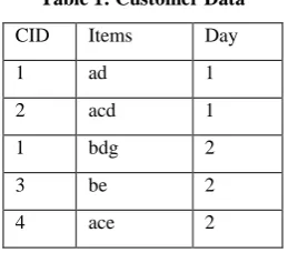
[image:1.595.364.494.649.763.2]E.g. consider the following customer bucket data:
Table 1: Customer Data
CID Items Day
1 ad 1
2 acd 1
1 bdg 2
3 be 2
2 be 3
3 af 3
1 c 4
3 cdg 4
4 df 5
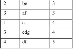
[image:2.595.103.231.72.158.2]Then from the above database one can make the following customer sequence database using above definition of sequence database.
Table 2: Sequence Database CID Customer Sequence
1 (ad)(bdg)(c )
2 (acd)(be)
3 (be)(af)(cdg)
4 (ace)(df)
Let min_sup = 2. The set of items in the above database is {a, b, c, d, e, f, g}. Database is consists of four sequences. The first sequence, namely < (ad)(bdg)(c) >, has three events (ad), (bdg) and (c). The length of this sequence is 6 (2+3+1). Sequence < (bg)(c) >is a subsequence of this sequence. Now consider the sequence < (ad)(b) >. Sequences 1 and 2 support this sequence and no other sequence support it. So its support count is 2, which satisfies minimum support threshold and hence this is a frequent sequence.
2. Need for Incremental Mining
Sequential mining algorithms can mine a static database. But, nowadays, almost all databases are dynamic in nature and they grow incrementally. One way to handle this is to mine the whole database every time an update occurs. But it is highly inefficient and also undesirable. We must find a way to use the already mined information. An incremental mining algorithm does the same. It utilizes the mined information to get new set of frequent sequential patterns instead of mining the whole database from scratch. Note that the ultimate aim of using an incremental mining algorithm instead of non-incremental one is to gain efficiency with respect to time. Otherwise a non-incremental mining algorithm can also serve the purpose of mining very easily. So for incremental mining algorithm the time takenby the algorithm to mine complete set of frequent patterns must be considered.
3. Incremental Mining of Sequential
Patterns
Given a sequence database D, a user-specified minimum support threshold, the set of frequent sequential patterns FP for D and an appended sequence database D’, the problem of incremental mining of sequential patterns is to mine the complete set of frequent sequential patterns for D’ using the already mined set of frequent patterns FP instead of mining D’ from scratch.
Now let us defines some terminology related to incremental mining and our approach.
Semi-frequent Pattern: Given a factor 0 < μ ≤ 1, a sequence
p is said to be semi-frequent if its support is less than min_sup but not less than μ*min_sup.
Boundary of Semi-frequent Patterns: It consists of the
frequent patterns which do not have its prefix as semi-frequent pattern.
Infrequent Pattern: A sequence p is said to be infrequent if
its support count is less than μ*min_sup.
Incremental Support of a Sequence: Incremental support of
a sequence is the increase of its support due to the update in database.
Appended Sequence: Given a sequence p = (p1p2…pk) and
another sequence q = (q1q2…qn), let p’ be the sequence obtained by concatenating q to p. Then p’ is called appended sequence of p. Note that if appended part is empty then we simply get p’=p.
Appended Sequence Database: An appended sequence
database D’ obtained from the database D is one with the following conditions:
i. For each sequence p’ in D’, there must exists a sequence p in D such that either p’ is appended sequence of p or p’=p.
ii. For each sequence p in D, there must exists a sequence p’ in D’ such that either p’ is appended sequence of p or p’=p.
LDB: LDB consists of those sequences of appended sequence
database D’ which have really got some appended part i.e. which are not equal to their corresponding sequence in original database D.
ODB: ODB consists of those sequences of original database D which have been appended with events in appended database D’.
Prefix: Given a sequence p = (p1p2…pn), a sequence p’ =
(p1’p2’…pm’) (m ≤ n) is called prefix of p if and only if (1) pi’ = pi for i ≤ m - 1; (2) pm’ ⊆ pm; and (3) all the items in (pm – pm’) are alphabetically (or according to the order specified) after the items in pm’.
Suffix: Let α = (pm’’pm+1…pn) be the sequence obtained from
the sequences p and p’ given in above definition such that pm’’ = (pm – pm’). Then α is called suffix or postfix of p with respect to p’.
Projection of a sequence: Given two sequences p and p’ such
that p’ is a subsequence of p, a subsequence α of the sequence p is called a projection of p with respect to p’ if and only if (1) α has p’ as its prefix and (2) there exists no other proper supersequence of α which is subsequence of p and has p’ as prefix.
Projected Database: Given a sequence p and a sequence
database D, the p-projected database is the collection of suffixes of sequences in D with respect to p.
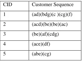
Table 3: Update to the database
CID Customer Sequence
1 (cg)(f)
2 (be)(ac)
5 (abe)(cg)
[image:3.595.90.231.263.369.2]So using above definition, one can find the appended database as:
Table 4: Appended Database
CID Customer Sequence
1 (ad)(bdg)(c )(cg)(f)
2 (acd)(be)(be)(ac)
3 (be)(af)(cdg)
4 (ace)(df)
5 (abe)(cg)
Also for above database and update, the LDB and ODB parts are given by the following tables.
Table 5: LDB
CID Customer Sequence
1 (ad)(bdg)(c) (cg)(f)
2 (acd)(be) (be)(ac)
[image:3.595.88.230.451.626.2]5 (abe)(cg)
Table 6: ODB
CID Customer Sequence
1 (ad)(bdg)(c)
2 (acd)(be)
Now suppose one wants to find the incremental support of < (a)(c) >.LDB is used for this purpose. It can be seen that customer sequences with CID 1, 2 and 5 support this sequence. But sequence with CID 1 in ODB also supports it. So sequence with CID 1 will not contribute to the incremental support of given sequence since it was already supported by this customer sequence in original database. Also note that it is not supported by sequence with CID 2 in ODB. So this sequence will contribute to the count. Same is the case with customer sequence with CID 5, since this is a new sequence representing a new customer.
4. Some Sequential Pattern Mining
Algorithms
GSP by Agrawal and Srikant: The term sequential pattern
mining is coined by Agrawal and Srikant (1995). They proposed three algorithms to solve the problem of finding frequent sequential patterns. Among these three algorithms AprioriAll was the best one. In 1996 they proposed another algorithm called GSP which outperform AprioriAll with a high degree. In GSP bottom-up approach is adopted to find the complete set of frequent sequential patterns. It finds frequent 1-sequences first, and then it generates candidate 2-sequences using the set of frequent 1-2-sequences. Then it finds frequent 2-sequences and so on. In general candidate k-sequences are generated using frequent (k-1)-k-sequences based on the anti-monotone property which states that all the subsequences of a frequent sequence must be frequent. After generating candidate sequences, the set of frequent sequences is determined by their support count. Frequent k-sequences are determined in the kth scan of the database and hence this algorithm requires as many database scans as the length of largest frequent sequence. So it is an algorithm which starts the sequential pattern mining and it can mine the complete set of frequent sequential patterns but it is not an efficient algorithm. So some researchers start thinking about efficient solution to this problem and proposed many algorithm, some of which we will discuss below.
SPADE: Another algorithm proposed by Zaki [6] called
SPADE is also based on the candidate generate and test approach. Zaki introduces the concept of lattice to divide the candidate sequences into groups such that each group can be completely stored in the main memory. In addition, this algorithm uses the ID-List technique to reduce the costs for computing support counts. An ID-list of a sequence keeps a list of pairs, which indicate the positions that it appears in the database. In a pair, the first value stands for a customer sequence and the second refers to a transaction in it, which contains the last itemset of the sequence.
The SPADE algorithm costs a lot to repeatedly merge the ID-lists of frequent sequences for a large number of candidate sequences. So, even if it is better than GSP but since it is also based on candidate-generate and test approach, it is also not very efficient. Thus more research work was needed to find some more efficient solution.
SPAM: To reduce this cost of merging, Ayres et al. [15]
adopt the lattice approach in the SPAM algorithm but represent each ID-list as vertical bitmap. The SPAM algorithm is efficient if all the bitmaps can be completely stored in the main memory. All the sequences are discovered in only three database scans. It outperforms GSP by a factor of two. But it has not shown much difference to SPADE.
PrefixSpan: Pei et al. [4] employ the projection scheme in the
projected database for each frequent k-sequence to find frequent (k+1)-sequences with this k-sequence as prefix. Obviously, the cost of PrefixSpan algorithm mainly depends upon the number of database projections to be generated recursively.
CloSpan: One other algorithm called CloSpan [9] is proposed
in 2003 keeping in mind the huge number of frequent sequences to be mined and stored. It mines the close sequential patterns i.e. the patterns which do not have a subsequence with same support count. Note that one can easily get the full set of frequent sequential patterns from the set of closed sequential patterns mined by CloSpan. So this algorithm turns out to be very good when minimum support is low i.e. when the number of frequent sequences is large.
Note that there are many other algorithms for mining sequential patterns but the above discussed algorithms represent the basic approaches.
5. Some Incremental Mining algorithms
ISM and ISE: Note that all the above discussed algorithms
can mine the set of frequent sequential pattern from a static database. But these days all real world databases are dynamic in nature. So, incremental mining algorithms came into existence. Incremental mining algorithm utilizes the already mined set of frequent sequential patterns for the original database to mine the complete set of frequent sequential patterns for the updated database. Parthasarathy et al. [7] proposed an incremental mining algorithm called ISM in which he used the concept of negative border. Negative border is defined as the set of sequences which are not frequent but both of whose generating subsequences are frequent. The generating subsequences of a sequence of length k are two subsequences of length (k-1) obtained by dropping exactly one of its first or second item. In this algorithm they have maintained a lattice of sequences to keep the set of frequent sequences and the negative border. This concept of negative border turns out to be helpful but it has its own drawbacks also. The main drawback of this approach is that the total number of sequences in the negative border is very large. So we have to store these infrequent sequences along with the set of frequent sequential patterns. Moreover the sequences in negative border may have very low support and they may not become frequent after many subsequent updates to the database. So there is no point in keeping those highly infrequent sequences. Later Masseglia et al. [13] proposed another incremental mining algorithm called ISE. In this algorithm the candidate-generate and test approach is used. The disadvantages of this algorithm include the huge number of candidate sequences to be tested and need of multiple scan of the whole database. So this algorithm turns out to be very costly with respect to time and space requirement.
IncSpan: Cheng et al. [2] proposed an incremental mining
algorithm called IncSpan based on an existing algorithm called PrefixSpan [4]. To gain efficiency the concept of semi-frequent patterns is introduced. Semi-semi-frequent patterns are the patterns which are not frequent but whose support is greater than the product of minimum support and a user specified factor μ (0 <μ < 1) i.e. patterns that are not frequent but are almost frequent. Note that these almost frequent patterns are most likely to be frequent in the updated database. The experimental results in [2] show that IncSpan outperforms the non-incremental algorithm PrefixSpan and an incremental mining algorithm ISM.
IncSpan+: Later Nguyen et al. [1] claimed that IncSpan
cannot mine the complete set of frequent patterns. They gave counter examples to justify their claim. They proposed an algorithm called IncSpan+ which is free from the shortcomings of IncSpan and can mine the complete set of frequent sequence patterns. They proved the correctness of IncSpan+.
6.
IncSpan+: An overview
IncSpan+ is proposed by Nguyen et al. in response to an incremental mining algorithm called IncSpan proposed by Cheng et al. [2]. IncSpan has a major drawback of not able to mine the complete set of frequent sequential patterns. It is observed by Nguyen et al. and they proposed the IncSpan+ algorithm which, they proved that, can mine the set of frequent sequential patterns completely. It adopts the same approach as IncSpan. It is also based on the PrefixSpan algorithm as IncSpan.
The IncSpan algorithm is given below:
Algorithm Outline: IncSpan+(D’, min_sup, µ, FS, SFS)
Input: An updated database D’, min_sup, FS and SFS in D
Output: FS’, SFS’ in D’
Method:
1: FS’ = Φ; SFS’ = Φ;
2: Determine LDB; Total number of sequences in D’, adjust
themin_sup if it ischanged due to the increasing of total
number of sequences in D’
3: Scan the whole D’ for new single items
4: Add new frequent items into FS’
5: Add new semi-frequent items into SFS’
6: For each new item i in FS’ do
7: PrefixSpan(i, D’|i, µ, min_sup, FS’, SFS’) 8: For each new item i in SFS’ do
9: PrefixSpan(i, D’|i, µ, min_sup, FS’, SFS’) 10: For every pattern p in FS or SFS do
11: Check Δsup(p) = supdb(p)
12: If supD’(p) = supD(p) + Δsup(p) ≥ min_sup 13: Insert(FS’, p)
14: If supLDB(p) ≥ (1 - µ) * min_sup
15: PrefixSpan(p, D’|p,µ,min_sup,FS’, SFS’)
16: ElseIfsupD’(p) ≥ µ * min_sup 17: Insert(SFS’, p)
18: PrefixSpan(p,D’|p,µ, min_sup,FS’, SFS’) 19: Return;
How it works: It takes as input, the Updated database D’, the
It initially sets FS’ and SFS’ to empty sets. Then it determines the LDB, which is set of those customer sequences that have got some appended part due to the update to the database. Then it finds the total number of sequences, which may have changed due to insertion of some new customer sequence. Also if the total number of sequences is increased, we have to adjust the min_sup also.
Then it scans the database D’ once to find out new frequent and semi-frequent single items and add them to FS’ or SFS’ accordingly. Note that here definition of new is crucial. In IncSpan [2] new single item is defined as the one which has no occurrence in the original database D and this proved to be a major shortcoming of IncSpan as later it was found that IncSpan cannot mine the complete set of frequent sequential patterns. It was due to this definition of new single items, since there may be some items, which are not new according to this definition i.e. which has there occurrences in D and are infrequent and after update to the database they might come up as frequent. E.g. suppose the minimum support required is 40 and the buffer ratio (μ) is 0.6 and there is a single item α having support count 20 in D and suppose it has got support count 40, as required to be frequent, in D’. Such types of patterns are not considered in IncSpan and this is the only reason for the incompleteness of the set of frequent sequential patterns. In IncSpan+, this weakness is observed and to rectify this flaw they defined new single items as the items which are not in FS or SFS i.e. which are not frequent or semi-frequent in D.
Now for each newly found frequent or semi-frequent item α,PrefixSpan is called to find out all the frequent or semi-frequent sequential patterns with prefix α.
After that, it considers the patterns in FS and SFS. Since one can find out all the frequent and semi-frequent sequential patterns with the help of patterns in FS and SFS, along with the previously found patterns, all one needs to do is to check the support count of these patterns to determine if they are frequent or not and call PrefixSpan on frequent ones and semi-frequent ones. But one needs not to call PrefixSpan for all of the frequent or semi-frequent patterns. For this it uses a pruning technique to reduce the calls to PrefixSpan. So it proceeds as follows.
For each pattern p in FS or SFS, first it checks its incremental support and adds it to its support in D to find its support in D’ i.e. first it updates its support. Then it checks if it is greater than min_sup or not. If it is found to be frequent according to new min_sup it is first added to FS’ and then its support in LDB is checked to determine if we have to call PrefixSpan or not based on the pruning condition it uses. On the other hand, if it is not found to be frequent but it is semi-frequent then simply it is added to SFS’ and PrefixSpan is called to find more frequent and semi-frequent sequential patterns. And the algorithm finishes its work.
7. Some Important Observations
1)One needs not to keep all the semi-frequent sequences. Suppose someone has a sequence α with him and some other sequence β has α as its prefix. Then he needs not to keep β, since he can always mine β with the knowledge of α. So if α is in SFS but β is not, there may be two situations about β:
β remains semi-frequent after the update.
In this case, there are two sub cases again. First, α becomes frequent after update. Then PrefixSpanis called on α and β can be found or its prefix to be semi-frequent and it can
be kept in SFS’ for future use. Secondly, α remains semi-frequent. Then one needs to do nothing as he will have α with him as before. Note that, for the patterns becoming frequent from SFS, one has to call PrefixSpan without checking the pruning condition to get the complete set of semi-frequent patterns for further updates to the database.
β becomes frequent after the update.
In this case, since α is prefix to β, α must have at least same supportcount as β and so α must be frequent. So PrefixSpan will be called on α and consequently get β.
2) One need not to check the pruning condition and call PrefixSpan (if required) on every sequence in FS and SFS. If only the length-1 sequential patterns of FS and SFSare considered, it will be sufficient. Suppose α is a length-1 sequential pattern and the pruning condition has been checked for it. Then either PrefixSpanis called on it or not. Now, if PrefixSpanis called on α, all the frequent patterns with prefix α are mined recursively and hence the patterns with α as prefix need not be considered. Also if PrefixSpan is not calledon α, then there is a guarantee that it will be not called on any pattern with prefix α. For this, note that PrefixSpan is called only if support of the pattern in LDB is greater than some fixed value ((1-μ)*min_sup). But, if it is not called for α means support of α is less than that. But, then support of a pattern having α as prefix is less than or equal to support of α and hence less than that fixed value.
3) Parthasarathy et al. [7] have used the concept of negative border in their algorithm ISM and Cheng et al. [2] have used the concept of semi-frequent sequential patterns in IncSpan. Both the algorithms have to store some non-frequent patterns. InMISP (Modified IncSpan+) both the concepts have been used.
Note that if one can keep the negative border completely, frequent sequential patterns can be mined very easily. The main problem with negative border is its huge size and highly infrequent patterns. Also it would be better if the number of semi-frequent sequential patterns can be reduced. One thing between negative border and semi-frequent patterns is common; patterns in both are either single items or have some frequent pattern as prefix. But not all semi-frequent patterns need to be in border since prefix of a semi-frequent pattern may itself be semi-frequent. Also, not all border sequences need to be semi-frequent due to their support count. So keeping the advantages of both the approaches in mind, MISP has been developed in whichthe intersection of the set of semi-frequent patterns and negative border is kept for future use. It is calledboundary of semi-frequent patterns. Asdiscussed above, it will be sufficient and very beneficial also for the time and space efficiency.
8. Our Approach: MISP (Modified
IncSpan+)
As stated before, it is modification to IncSpan+ and so it follows the same spirit. The algorithm is presented first and then it is discussed. The algorithm is:
Input:An appended database D’, min_sup, FP and BSFP in D
Output: FP’, BSFP’ in D’
Method:
1: FP’ = Φ; BSFP’ = Φ;
themin_sup if it ischanged due to the increasing of total
number of sequences in D’.
3: Scan the whole D’ for new single items
4: Add new frequent items into FP’
5: Add new semi-frequent items into BSFP’
6: For each new item i in FP’ do
7: PrefixSpan(i, D’|i, µ, min_sup, FP’, BSFP’) 8: For every pattern p in FP do
9: Check Δsup(p) = supdb(p)
10: If supD’(p) = supD(p) + Δsup(p) ≥ min_sup 11: Insert(FP’, p)
12: If supLDB(p) ≥ (1 - µ) * min_sup&& (p is a single item)
13:PrefixSpan(p, D’|p, µ, min_sup, FP’, BSFP’)
14: ElseIfsupD’(p) ≥ µ * min_sup
15:Insert(BSFP’, p)
16: For every pattern p in BSFP do 17: Check Δsup(p) = supdb(p)
18: If supD’(p) = supD(p) + Δsup(p) ≥ min_sup 19: Insert(FP’, p)
20: PrefixSpan(p, D’|p, µ, min_sup, FP’, BSFP’)
21:ElseIfsupD’(p) ≥ µ * min_sup
22: Insert(BSFP’, p)
23: Return;
9. Working of MISP
MISP and IncSpan+ are almost same except the following modifications:
1. In MISP,PrefixSpanneed not be called for the new semi-frequent single items, since only the boundary is kept. (See line 8-9 in IncSpan+)
2. In MISP, the patterns of FS and SFS are considered separately, since for patterns of SFS, which becomes frequent after update, PrefixSpan is called without checking pruning condition so that one can get the complete boundary of semi-frequent patterns.
3. For patterns of both FS and SFS, which becomes semi-frequent from frequent due to the change in min_sup or which remains semi-frequent, PrefixSpan is not called. (See line 18 in IncSpan+)
4. Also for patterns of FS, which becomes frequent after update and also satisfy the pruning condition,PrefixSpan is not called all the time. Instead, it is called only for single such items.
Note that if the database is projected physically then very much memory space is required.
Since PrefixSpan is called recursively and so the database needs to be projected recursively. So they have to be stored on disc. Also reading and writing from and to the disc is much
slower than from main memory. So this may be major cost for the algorithm if the number of projected databases is large and they have to be projected physically. So somehow if the size of these projected databases is kept small, they can be stored to the main memory. So the approach of not projecting the database physically as in PrefixSpan called
pseudo-projectionis applied in which the sequence index and the
starting position of the projected sequenceis kept. The size of such a record is significantly less than that of physically projected database and so it can be kept in main memory.
To further illustrate the working of both the algorithms, they are applied to an example database below.
10. Example:
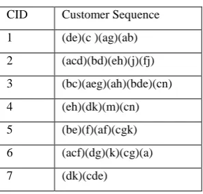
[image:6.595.342.482.284.408.2]Suppose the following data is given as original customer sequence database:
Table 7: Customer Sequence Database D
CID Customer Sequence
1 (de)(c )(ag)(ab)
2 (acd)(bd)
3 (bc)(aeg)(ah)
4 (eh)(dk)(m)(cn)
5 (be)(f)(af)(cgk)
6 (acf)(dg)(k)
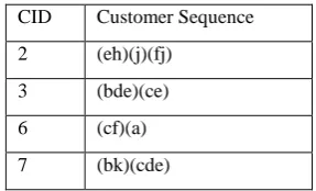
And suppose the update is given as:
Table 8: Update Part δD
CID Customer Sequence
2 (eh)(j)(fj)
3 (bde)(ce)
6 (cf)(a)
7 (bk)(cde)
Also suppose that minimum support threshold is 0.66, the buffer ratio μ is 0.6. Total number of customer sequences is 6 and so min_sup is 4. So the set of frequent sequential patterns FS and set of semi-frequent sequential patterns SFS for D are given by
FS = {< (a) : 5 >, < (b) : 4 >, < (c) : 6 >, < (d) : 4 >, < (e) : 4
>, < (g) : 4 >}
SFS = {< (c)(g) : 3 >, < (e)(a) : 3 >, < (e)(c) : 3 >, < (k) : 3 >}
[image:6.595.340.484.486.573.2]Table 9: LDB Part
CID Customer Sequence
2 (acd)(bd)(eh)(j)(fj)
3 (bc)(aeg)(ah)(bde)(cn)
6 (acf)(dg)(k)(cf)(a)
7 (bk)(cde)
And then appended database D’ is made with the help of original database D and the update part δD as given below:
Table 10: Appended Database D’
CID Customer Sequence
1 (de)(c )(ag)(ab)
2 (acd)(bd)(eh)(j)(fj)
3 (bc)(aeg)(ah)(bde)(cn)
4 (eh)(dk)(m)(cn)
5 (be)(f)(af)(cgk)
6 (acf)(dg)(k)(cg)(a)
7 (dk)(cde)
After this, IncSpan+ will scan the appended database D’ once to find out new single frequent or semi-frequent items. The only new single item found in this case is (h) with support count 3 and so it is semi-frequent. So it is added to SFS’ to get
SFS’ = {< (h) : 3 >}.
Then PrefixSpan is called on (h) but no other semi-frequent pattern was found. Obviously, we cannot get semi-frequent patterns on calling PrefixSpan on a semi-frequent pattern.
Now, it considers the patterns of FS and SFS one by one to check their support count and calling PrefixSpan if necessary. If a pattern is found to be frequent, it is added to FS’ and if it is found to be semi-frequent it is added to SFS, otherwise it is just discarded. Note that the whole database need not to be scanned to check the support count of these sequences since the incremental support can be find out with the help of LDB andtheir support in original database is already stored with them in FS or SFS. So the scan of the database is needed only if PrefixSpanis called to find more patterns. So when this algorithm returns, the set of frequent sequential patterns FS’ and set of semi-frequent sequential patterns SFS’ will be as
FS’ = {< (a): 5 >, < (b) : 5 >, < (c) : 7 >, < (d) : 6 >, < (e) : 6
>}
SFS’ = {< (a)(a) : 3 >, < (a)(b) : 3 >, < (a)(c) : 3 >, < (a)(d) : 3
>, < (b)(c) : 3 >, < (b)(e) : 3 >, < (c)(a) : 3 >, < (c)(b)
: 3 >, < (c)(d) : 3 >, < (c)(g) : 3 >, < (c)(g)(a) : 3 >, <
(d)(c) : 4 >, <(de) : 3 >, < (e)(a) : 3 >, < (e)(c) : 4 >,
< (f) : 3 >, < (h) : 3 >, < (g) : 4 >, < (g)(a) : 3 >,
< (k) : 4 >, < (k)(c) : 3 >}
Note that (g) was a frequent pattern before update but it is no more frequent after update. Also so many new patterns have come.
Now MISP algorithm is applied to the above
example database and update part. The adjustment of
min_sup, making of LDB and D’ will be same. They will be same as shown above in Table 3 and Table 4. Also, by chance, BSFP also found to be same as SFS for this particular data. Most of the times, they differ.
Now MISP finds the new frequent and semi-frequent single items. As in IncSpan+, it finds (h) as new semi-frequent single item. But, it does not call PrefixSpan on it as IncSpan+ does. So this is the first difference we have encountered.
Then MISP considers the patterns of FP. Here it continues same as IncSpan except that it does not call PrefixSpan for the semi-frequent sequential patterns. Also it does not call PrefixSpan on patterns of length more than 1. For patterns of BSFP, it calls PrefixSpan only if the pattern has becomes frequent. If it remains semi-frequent it simply adds it to BSFP’. Also if due to the change in min_sup if a pattern has becomes infrequent, we simply leave it.
So at last MISP finds the following set of frequent sequential patterns and BSFP
FP’ ={< (a): 5 >,< (b) : 5 >, < (c) : 7 >, < (d) : 6 >, < (e) : 6 >}
BSFP’ = {< (a)(a) : 3 >, < (a)(b) : 3 >, < (a)(c) : 3 >, < (a)(d) :
3 >, < (b)(c) : 3 >, < (b)(e) : 3 >, < (c)(a) : 3 >, <
(c)(b) : 3 >, < (c)(d) : 3 >, < (c)(g) : 3 >, < (d)(c) : 4
>, < (de) : 3 >, < (e)(a) : 3 >, < (e)(c) : 4 >, < (f) : 3
>, < (h) : 3 >, < (g) : 4 >, < (k) : 4 >}
Note that this time BSFP’ and SFS’ are not the same. BSFP’ has fewer elements. Note that the patterns< (c)(g)(a) : 3 >, < (g)(a) : 3 > and < (k)(c) : 3 > are not stored since < (c)(g) : 3 >, < (g) : 4 > and < (k) : 4 >are in BSFP’. Also note that, FS’ and FP’ are exactly the same i.e. MISP can mine the same set of frequent patterns as IncSpan+.
11. Experimental Results
MISP and IncSpan+ are compared for various attributes on a set of customer data and the results found are as follows:
[image:7.595.86.235.277.419.2]Note that MISP outperforms IncSpan+ when the minimum support is low and the number of frequent sequential patterns is high with a wide margin. Even if the minimum support is not low, it is somewhat efficient than IncSpan+.
The chart below shows the number of calls to a function PrefixSpan required by the algorithms for various minimum supports.
Note that in MISP,PrefixSpan is called remarkably less number of times than in IncSpan+. This is the key factor to performance since in every call to PrefixSpan the database is scanned once and on the semi-frequent patterns, one also has to project the database. So number of calls to PrefixSpan is directly proportional to number of database scans required. Actually number of calls to the PrefixSpan is equal to the database projection required. Also it is directly proportional to the database projections. So fewer calls to PrefixSpan means fewer database scans, fewer database projections and hence less time requirement keeping in mind that it takes considerable time to scan a database and project the database.
The chart below shows the number of semi-frequent patterns to be required to store by the algorithms on varying minimum support threshold.
Note that in MISP algorithm one has to buffer less number of semi-frequent patterns and hence required less memory. Also, the number of semi-frequent sequential is directly proportional to the number of calls to the PrefixSpan algorithm in IncSpan+. So it is directly proportional to the database scans and hence causes large number of database projections. So it increases the overhead of projecting the database significantly.
12. Conclusion
In this work, we have proposed an algorithm called MISP for incremental mining of sequential patterns. It is a modification to an existing algorithm called IncSpan+ for its efficiency with respect to time and space. Our experimental results show that we have succeeded in our goal up to some extent. For large database with a lot of frequent patterns, our algorithm is very efficient. If the minimum support threshold is low, which means the number of frequent patterns is huge, then
IncSpan+ algorithm has to call the PrefixSpan method a
large number of times and hence it has to scan the database a large number of times. Also scanning the whole database requires considerable amount of time. So we have attacked the problem of efficiency by reducing the number of calls to the
PrefixSpan method which in turn reduces the number of
database scans and therefore increases efficiency. Note that we have also reduced the number of semi-frequent patterns to be stored slightly resulting in less overhead of storing the non-desirable information, since we are interested in the frequent patterns only. So MISP required less number of infrequent patterns to be stored to find the frequent patterns in next update.
13.
Future Scope
A new concept of “time-interval sequential patterns” has been proposed recently in which not only the order of events but the time between them is also considered. This work can be further extended to develop an incremental mining algorithm for time-interval sequential patterns. The concept of
closed sequential patterns is not new these days. Closed
sequential patterns represent the information in more compact way and so they have gained much attention of the researchers. So an enthusiastic researcher can also try to develop an efficient algorithm for closed sequential patterns.
14. References
[1] Nguyen S.N., Sun X., Orlowska M.E., “Improvements of IncSpan: Incremental Mining of Sequential Patterns in Large Database”, Proc. of the 9th Pacific-Asia Conference on Advances in Knowledge Discovery and Data Mining, 2005.
[2] Cheng H.,YanX.,Han J., “IncSpan: Incremental Mining of sequential Patterns in large database.Proc. ACM KDD Conf. on Knowledge Discovery in Data, Washington (KDD’04).2004.
[3] Agrawal R., Srikant R.: Mining sequential patterns. Proc. 11th IEEE Int. Conf. on Data Engineering (ICDE’95),1995.
[4] Pei J., Han J., Mortazavi-Asl B., Wang J., Pinto H., Chen Q., Dayal U., Hsu M.: Mining sequential patterns by Pattern-Growth: The PrefixSpan approach. IEEE Transactions on Knowledge and Data Engineering, Vol.16, No. 10, 2004.
0 20 40 60 80 100
0.5 0.45 0.4 0.35 0.3 0.25 0.2
T
im
e
in
s
ec
o
n
d
s
Minimum support threshold
IncSpan+
MISP
0 20 40 60 80
0.5 0.45 0.4 0.35
N
u
m
b
er
o
f ca
lls
Minimum support count
IncSpan+
MISP
0 50 100 150
0.5 0.45 0.4 0.35 0.3
N
u
m
b
er
o
f se
m
i f
re
q
u
en
t
p
at
te
rn
s
Minimum support count
IncSpan+
[5] Srikant R., Agrawal R.: Mining sequential patterns: Generalizations and performance improvements. Proc. 5th IEEE Int. Conf. on Extending Database Technology (IDBT’96).
[6] Zaki M.: SPADE: An efficient algorithm for mining frequent sequences,Machine Learning, 40: (31-60), 2001
[7] Parthasarathy S., Zaki M., Ogihara M., and Dwarkadas S.: Incremental and interactive sequence mining. Proc. 8th Int. Conf. on Information and Knowledge Management (CIKM’99), 1999.
[8] Zhang M., Kao B., Cheung D., Yip C.: Efficient algorithms for incremental update of frequent sequences. Proc. of Pacific-Asia Conf. on Knowledge Discovery and Data Mining (PAKDD’02), 2002.
[9] X. Yan, J. Han, and R. Afshar.Clospan: Mining closed sequential patterns in large datasets, 2003.
[10] J. Han, J. Pei, B. Mortazavi-Asl,Q. Chen, U. Dayal, and M.C Hsu, ”FreeSpan: Frequent Pattern-Projected Sequential Pattern Min- ing,"Proc.2000 ACM SIGKDD Int'l Conf. Knowledge Discovery in Databases (KDD '00),pp. 355-359,Aug. 2000.
[11] I.H. Witten, and F. Frank,Data Mining: Practical Machine Learning Tools With Java
Implementations.,San Francisco, CA: Morgan Kauf- man,2000.
[12] Dao-I Lin, and Zvi M. Kedem, “Pincer Search: An Efficient Algorithm For Discovering The Maximum Frequent Set," IEEE Trans. on Knowledge and Data Engineering, Vol. 14, No. 3, (May/June, 2002), pp. 553-566.
[13] F. Masseglia, P. Poncelet, and M. Teisseire. Incremental mining of sequential patterns in large databases. Data Knowl. Eng., 46:97–121, 2003.
[14] F. Masseglia, P. Poncelet, M. Teisseire, “Incremental mining of sequential patterns in large databases,” Actes des Jouenes Bases de DonnesAvances (BDA’00), Blois, France, 1999.
[15] J. Ayres, J. E. Gehrke, T. Yiu and J. Flannick, “ Sequential pattern mining using bitmaps.”, Proc. 2002 ACM SIGKDD Int. Conf. Knowledge Discovery in Databases (KDD’02), July 2002.
[16] Jiawei Han and MichelineKamber, “Data Mining: Concepts and Techniques”, 2nd