Munich Personal RePEc Archive
A Threshold Cointegration Analysis of
Asymmetric Adjustment of OPEC and
non-OPEC Monthly Crude Oil Prices
Ghassan, Hassan B. and Banerjee, Prashanta K.
Umm Al-Qura University (Department of Economics), Institute of
Bank Management (Department of Research, Development
Consultancy)
3 October 2013
Online at
https://mpra.ub.uni-muenchen.de/65672/
0
A Threshold Cointegration Analysis of Asymmetric
Adjustment
of OPEC and non-OPEC Monthly Crude Oil Prices
Hassan Belkacem Ghassan
Prashanta Kumar Banerjee
Department of Economics
Department of Research, Development & Consultancy
Umm Al-Qura University, Saudi Arabia
Institute of Bank Management, Bangladesh
Abstract
The purpose of this paper is to analyze the dynamics of crude oil prices of OPEC and non-OPEC
countries using threshold cointegration. To capture the long run asymmetric price transmission
mechanism, we develop an error correction model within a threshold cointegration and CGARCH errors
framework. The empirical contribution of our paper specifies the cointegrating relation between OPEC
price and non-OPEC prices and estimates how and to what extent the respective prices adjust to eliminate
disequilibrium. The finding exhibits that the conditional volatility of variance has long run memory
feature and the shocks on the long run component do not adjust quickly. The OPEC producers could not
drive down (up) crude oil prices with equivalent speeds for all participants in the market. The slow
adjustment of OPEC process of positive discrepancies to the long run equilibrium indicates that OPEC
does not prefer modest oil prices. While, the rapid adjustment of non-OPEC process signifies their
preference of modest oil prices after oil price increases. These differences of speeds show evidence for
competitive behaviors between OPEC and non-OPEC countries.
Key words: Asymmetric adjustment, CGARCH, OPEC prices.
1
1. Introduction
Oil is one of the world’s largest traded commodity, most of the international flow of funds moves around
this commodity. And everybody is far more aware of changes in its price. Therefore, the price of oil is
always under public scrutiny. The price was stable near $3 per barrel before 1970. Afterwards, the Arab
oil embargo, the crises in Iran and Iraq, the recent crises in the Middle East and, importantly, the
increasing demand of growing economies like China, India have impacted on the prices of oil, which
reached a record level of $145 per barrel in 2008. Changes in the price of oil are overwhelmingly
significant because it drives national and international economic and military policies around the world.
Therefore, the analyses of the price of oil always have been significant interest to academics, bankers,
business people and policy makers alike.
The Organization of Petroleum Exporting Countries (OPEC), which was established in 1960, and
often treated as a monopoly and a cartel, has had mixed success in controlling prices. OPEC might
exercise great influence over the world prices of oil, because the member countries have enough spare
capacity of oil. The non-OPEC countries have an excess demand of approximately 33 million barrels per
day (Appendix Table A), even though their share is as high as 60 per cent in the total world production of
oil (Appendix Table B). This entire excess demand of non-OPEC countries is satisfied with the oil
supplied by the OPEC countries only. As a result, it is a common belief that the non-OPEC countries
behave as price takers and the OPEC might play a dominant role in the world by setting the price of oil by
adjusting its production.
A large body of literature is available on the price of oil. Gately (1993) examines the price
reversibility of world oil demand using price decomposition methods. He finds that the reductions in the
world demand for oil following the oil price increases of the 1970s have not been completely reversed by
the price cuts of the 1980s.The response to price cuts in the 1980s equates to only one –fifth of the total
price increases in the 1970s. De Santis (2003) seeks to explain the crude oil prices fluctuations by
2
observes that Saudi Arabia’s behavior is asymmetric in response to the world demand shocks because
they have an incentive (disincentive) to intervene if negative (positive) demand shock hits the crude oil
market. Jones (1990) studies OPEC behavior under falling prices and shows evidence of oil price
reductions being more the result of deliberate output adjustments by the cartel, not of an unintentional
outcome of a breakdown in cartel discipline that may eventually cause its collapse. Lin (2009) finds an
oligopolistic behavior among non-OPEC producers and collusion among OPEC producers during the
period 1970-2004. In addition, Hamilton (2008) examines the factors responsible for changes in crude oil
prices by reviewing the statistical behavior of oil prices, relating them to the predictions of theory, and
investigates in details the key features of petroleum demand and supply. He concludes that although
scarcity rent made a negligible contribution to the price of oil in 1997, it could begin to play a role. Li
(2010) shows that the flow of causation runs from non-OPEC production to the world oil prices and then
to OPEC production. This is a complete reversal of what one would expect if OPEC were influential in
the world oil market. This indicates that it is not appropriate to treat OPEC as a dominant firm. Apart
from these, many empirical studies are conducted on supply and demand in the petroleum market (see
e.g., Adelman 1962; Kennedy 1974; Berndt & Wood 1975; Hausman 1975; Nordhaus 1980; Gately 1984;
Griffin 1985; Goldberger 1991; Manski 1995; Angrist et al. 2000; Gately & Huntington 2002; Lin 2009).
Most of the previous work assumes that the adjustment process is strictly symmetric. Now, it is
widely acknowledged that many important economic variables display asymmetric adjustment paths.
Moreover, a number of studies claim that there is an asymmetric relationship between the oil price
followed by OPEC and non-OPEC countries (Ewing et al. 2006; Bekiros et al. 2008; Kang et al. 2009;
Mohammadi et al. 2010; Hammoudeh et al. 2010). Chen et al. (2005) documented new supportive
evidence for asymmetric adjustment in the United States retail gasoline prices. However, the local market
price is a different story because it is affected by the sales tax and domestic oil reserves, especially within
the United States. The asymmetric transmission is found to occur not just through the spot markets of
crude oil and refinery gasoline, but also through their future markets. It also shows that the observed
3
process.Lastly, Balke et al. (1998) use several different model specifications to analyze the relationship
between the oil prices and the spot, wholesale, and retail prices of gasoline. They find asymmetry is
sensitive to model specification, but is pervasive in the most general model. A number of empirical
studies have also been conducted on price asymmetry for North American markets, but the findings of
these studies are mixed (Borenstein et al. 1997; EIA 1999; Godby et al. 2000).
The purpose of this paper is to analyze the dynamics of oil prices of OPEC and non-OPEC countries
in the international market. The aim is to reveal whether the prices of oil for both groups are cointegrated,
either the price adjustment process is symmetric or asymmetric, and to determine whether any causality
relationship exists among the two different oil prices. Given the perception that exists regarding the
oligopolistic nature of the oil market, the paper aims to test for the presence of cointegration in the
presence of the asymmetric error correction across the oil prices followed by OPEC and non-OPEC
countries. The correspondence between error correction models, which represents cointegrating
relationships and autoregressive models of an error term, allows us to apply the method suggested by
Enders and Siklos (2001). Hence, the threshold autoregressive (TAR) and momentum-threshold
autoregressive (MTAR) method of adjustment are followed here.
The paper is organized as follows: Section 2 describes the methodology used, Section 3 reports the
description of the data and the empirical findings, and Section 4 concludes.
2. Methodology
First, the Engle and Granger (1987) two-step method is employed to test cointegration between the oil
prices of OPEC and non-OPEC countries. The price of oil of the OPEC and non-OPEC countries is
represented by
and
, respectively. This entails using ordinary least squares to estimate the long-runrelationship, which is given by the following:
4
After obtaining the estimated residuals from the equation 1, the ADF test is used on the resulting
residuals,
, to illustrate the cointegrated relationship between these two variables. This is illustrated by
the following equation:
(2)
where is a white noise error term. If the residuals retrieved from the equation (1) is stationary, then the
null hypothesis of no cointegration is rejected. However, Enders and Siklos (2001) argue that the test for
cointegration and its extensions are mis-specified if adjustment is asymmetric. They proposed the
following asymmetric adjustment, called the threshold autoregressive (TAR) model:
(3)
where and are the speed–adjustment coefficients and is the indicator function, which is defined
as the following:
(4)
This indicator function indicates that signifies adjustments from below the threshold (widening),
because the residual is expanding or greater than the threshold. The opposite holds true for
: the
adjustment is from above the threshold or the spread is narrowing.
This specification allows for asymmetric adjustment. If the system is convergent, then the long-run
equilibrium value of the sequence is given by which can be 0.1 The sufficient conditions for the
stationarity of
are
,
and
(Petrucelli and Woolford 1984). In
this case, if
is above its long-run equilibrium value, then adjustment is at the rate
, and if
is
below long-run equilibrium, then the adjustment is at the rate . This adjustment would be symmetric if
. However, if the null hypothesis Ho:
is rejected, then using the TAR model, we can
capture the signs of asymmetry. For example if
, then the negative phase of the
1
5
series will tend to be more persistent than the positive phase.i In the above case, it is necessary to estimate
the threshold value that will be equal to the cointegrating vector. A method of searching for a consistent
estimate of the threshold was undertaken by using a method proposed by Chan (1993).
Enders and Siklos (2001) suggest a further alternative such that the threshold depends on the
previous periods change in
instead on the level of
. In this case, the indicator can be set as follows:
(5)
The series
exhibits more momentum in one direction than the other. The model given by (3) along
with the equation (5) depicts the momentum threshold auto regression (MTAR) model. The MTAR can
be used to capture different types of asymmetry. For example, if
, then the MTAR exhibits
little adjustment for positive
, but substantial decay for negative
. In other words, increases
tend to persist, but decreases tend to revert quickly back to the attractor irrespective of where
disequilibrium is relative to the attractor. As before, the threshold for this model is estimated using
Chan’s methodology.
In this test, to implement the case of the TAR or MTAR adjustment, the indicator function is set
according to Eq. (4) or Eq. (5), respectively, and the estimate of Eq. (3) accordingly. The -statistic for
the null hypothesis of non-stationarity of
, i.e. under Ho:
,
has a unit root. The value
of the -statistic is compared to the critical values computed by Enders and Granger (1998). If we can
reject the null hypothesis, it is possible to test for asymmetric adjustment because and converge to a
multivariate normal distribution (Tong 1990). The -statistic is used to test for the null hypothesis of
symmetric adjustment, that is, Ho:
. Diagnostic checking of the residuals are undertaken to
ascertain whether the series has auto-correlation process using the Durbin-Watson test.
The finding of cointegration with threshold adjustment justifies the estimation of the following error
correction model with a threshold adjustment. The error correction model with a threshold cointegration,
6
(6)
where the variables and represent the error correction terms,
defined from the indicator functions in Eq. (4) and (5).2 The coefficient captures the speed of
adjustment or rate of convergence from gravitates back toward the long-run equilibrium path. In case of
i.e. undervaluation of the current crude oil prices, we expect that would be negative, therefore
leading to a downward adjustment. In case of i.e. overvaluation, we expect that would be negative, which conducts to an upward adjustment to converge to the long-run equilibrium. If the
convergence condition is verified i.e. , when ( ), we will have an upward
(downward) adjustment. The stochastic error is supposed to be distributed following the specific
component GARCH (CGARCH) errors Eq. (7), which are used particularly in financial applications
(Gospodinov 2008). This framework, named ECM-TAR-CGARCH, leads to a parsimonious
representation of some stylized features of the OPEC and non-OPEC prices such as the time-varying
volatility and the volatility clustering. The lag numbers are determined using the information criteria such
AIC and T-sig. The structure of errors is determined by the following equations:
and (7)
(8)
(9)
where is a stochastic process of the independently and identically distributed error term. The Eq. (8) of
the conditional variance exhibits the long-run component and the short-run component .
This transitory component contains the discrepancies around the long run component. Engle and Lee
(1999) point out that the CGARCH process, defined in separated equations (8) and (9), is weakly
stationary if and .3 The CGARCH model captures the volatility persistence of the
2
In the TAR adjustment, we have and ; while in the MTAR adjustment: and .
3
7
transitory and permanent dynamics. The long run trend of the conditional variance indicates the idea of
time-varying long run volatility. The parameter represents the decay rate and specifies the speed of the
mean reversion, which assumes that the high and lower crude oil prices are temporary. Therefore, it is
expected that the high and lower deviations, due to diverse shocks in the prices, will go back to an
average price. The conditional variance displays the long run mean reversion to a constant level given by
the unconditional variance . The volatility prediction error has zero-mean and serially
uncorrelated; it drives the dynamics of the permanent component (Poon et al. 2006). The strength of
shocks to the permanent component is defined by
. The shocks to the transitory component
revert to the trend , while in the GARCH model the shocks decay to the unconditional variance
. The power of shocks to the transitory component is determined by
. The
permanent process has memory close to unit root when is close to 1.4 Typically is between 0.9 and
1 (Table 4), then tends to its unconditional variance very slowly, this is due to the slow adaptation
to news. If , the transitory mean reverting process has more rapid time decay governed by
. If the conditional variance mean-reverts to a long-run trend level with the speed
determined by . It is assumed that when , then the permanent component is more
persistent than the transitory component. The persistence in the transitory component is lower than the
persistence in the permanent component, because . Consequently, the permanent component
has a long memory, whereas the transitory component has a short memory (Ray and Tsay 2000).
The volatility persistence of transitory large shocks is shorter than shocks due to habitual news
events, but it remains that the large shocks could have a permanent impact. Albeit with the CGARCH
structure, the parameters do not have all non-negative signs. The transitory component could be negative,
without the conditional variance becoming negative, suggesting the shocks on the volatility during the
convergence of the long-run trend. These volatility shocks lead to an uncertain future evolution,
4
8
indicating the presence of the volatility clustering (Engle and Patton 2000), which means that when the
negative news happens during the prices increase, the volatility also increases.5
In the component GARCH model, which is designed to capture the long memory of volatility, a
shock in the volatility series appears to have a long memory, and impacts on future volatility over a long
temporal horizon. When the autoregressive root ,6 the unconditional variance does not exist i.e. there is no mean reversion, but a shock remains through conditional variance and impacts upon future
volatility over an infinite horizon (Bollerslev and Engle 1993). The CGARCH process is covariance
stationary, when the conditional variance is stationary; and then both the permanent and transitory
components must both be covariance stationary, which necessitates and (Engle and Lee 1999).
3. Data and Empirical Results
The study is based on the monthly data on the per barrel price of crude oil in US Dollar in both OPEC and
non-OPEC countries. Both variables are converted into natural logs, and these variables are given a new
name: LOPEC and LNOPEC. The averages of OPEC and non-OPEC prices are based on the affiliations
of the countries for the stated period of time that may differ from current affiliations. The monthly data
are based on FOB prices from the first business day of the first week. OPEC and non-OPEC prices are
calculated as the average price (FOB) weighted by the export volume. To avoid the structural changes
that occurred during the 1970s and 1980s, our sample monthly data (Appendix, Figures 1) cover the
period January 1997 through April 2011. The data are gleaned from US Energy Information
Administration and the link used for collecting these data is as follows:
http://www.eia.gov/dnav/pet/pet_pri_wco_k_w.htm.
5
This phenomenon appears when the differences in the interpretability of information from the crude oil market accentuate the competitiveness between the OPEC and non-OPEC producers.
6
9
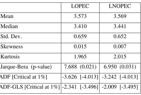
The mean to median ratio of each variable (Table 1) apparently indicates that the distribution of the
variable is not far from a symmetrical distribution as this ratio is close to one7. We expect that the crude
oil prices do not follow an independent and identically distribution. If the random variables are
independent, then the unconditional distribution is equal to the conditional distribution. But, the temporal
dependence doesn’t allow the independence feature even in the normal distribution, it makes more
interesting for the conditional distribution. Then, the empirical analysis is focused on the unconditional
distribution of the crude oil prices, based on past information and requiring stable processes. However,
the standard deviation, skewness and kurtosis fail to confirm the normality of each variable. The
distribution of monthly data of crude oil prices exhibits a positive skewness and a positive excess
kurtosis; it appears that we have a leptokurtic distribution. The Jarque-Bera statistics, as parametric test,
[image:11.612.184.431.365.532.2]clearly reject the null hypothesis of a normal distribution.
Table 1: Descriptive Statistics and Unit Root Tests
LOPEC LNOPEC
Mean 3.573 3.569
Median 3.410 3.441
Std. Dev. 0.659 0.652
Skewness 0.015 0.007
Kurtosis 1.965 2.015
Jarque-Bera (p-value) 7.688 (0.021) 6.950 (0.031)
ADF [Critical at 1%] -3.626 [-4.013] -3.242 [-4.013]
ADF-GLS [Critical at 1%] -2.341 [-3.496] -2.009 [-3.495]
To determine the order of integration, both oil prices were initially tested by using the ADF and
ADF-GLS with traditionaland Modified AIC and SIC. The ModifiedAIC, suggested by Ng and Perron (2001),
improves the size and power of the test. These statistics suggest that the OPEC and non-OPEC prices
7
10
have unit root process, but are stationary in their first difference term. In addition, when the variables are
I(1), the unconditional distribution may not exist. Of course, the underlying stochastic process cannot lead
to the leptokurtic unconditional distribution if the process is not strictly stationary. Plots of the first
difference of the logged crude oil prices (Appendix, Figures 1) exhibits a conditional heteroscedasticity,
but it does not mean necessarily that the series are from leptokurtic conditional distribution. So, the
unconditional leptokurtosis could reflect conditional heteroscedasticity. A GARCH model may be enough
for this purpose to capture the fat-tailedness of the unconditional distribution (Diebold & Lopez 1995,
Engle & Gonzalez-Rivera 1991). The movement of non-OPEC prices does not occur in isolation, but they
cluster with OPEC prices. The presence of the volatility clustering would justify to model in the
CGARCH framework (Engle and Patton 2000).8
3.1 Cointegration tests
To determine the long-run equilibrium relation between OPEC price and non-OPEC prices, both Engle
and Granger’s (EG, 1987) and Perron and Rodriguez’s (PR, 2001) methods have been implemented using
the software GAUSS. Both tests assume only a symmetric adjustment. Because the visual data do support
a constant and trend, each cointegration test includes a constant and trend as deterministic components.
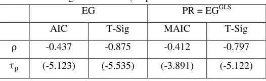
For the estimation of the EG, the AIC and T-significance are used to choose the lag order. The results in
Table 2 show that the EG test rejects the null hypothesis of no cointegration at the 5% and 1% level,
respectively, in accordance with the AIC and T-significance criteria. This illustrates that there is a
plausible cointegration relationship between the oil-selling price determined and followed by OPEC and
non-OPEC countries. Additionally, the PR test supports the findings of the EG test and rejects the null
hypothesis of no cointegration at the 1% level for both the AIC and T-significance criteria.
8
11
Table 2a: Cointegration Tests (Dependent Variable LOPEC)ii
EG PR = EGGLS
AIC T-Sig MAIC T-Sig
-0.499 -0.855 -0.396 -0.742
[image:13.612.175.438.185.265.2](-3.954) (-5.477) (-3.789) (-4.946)
Table 2b: Cointegration Tests (Dependent Variable LNOPEC)
EG PR = EGGLS
AIC T-Sig MAIC T-Sig
-0.437 -0.875 -0.412 -0.797
(-5.123) (-5.535) (-3.891) (-5.122)
In the EG method, if the variables are interchangeable and the sample size is sufficient, then the same
results will be attained (Table 2a and Table 2b). According to Horvath & Watson (1995) when there is
only one cointegrating vector, simple univariate tests provide an alternative to the likelihood-based tests.
They conclude that the power trade-off between the multivariate and the univariate tests for cointegration
is more interesting in higher dimensional systems.
In our case, the Johansen test justifies that the logged price series of OPEC and non-OPEC move
together towards a one stable long run relationship. 9 We find a significant trace-statistic with 26.96 and a
significant max-eigen statistic with 26.06, the critical values at 1% are 19.94 and 18.52, respectively. By
running the causality test, from VEC model instead of VAR model, using -statistic, we find a causality
from OPEC prices to non-OPEC prices, where with p-value equal 0.084.
The statistic of Stock & Watson (1988) tests the null hypothesis of stochastic trends of series
against their common trends i.e. cointegrated series10 in the multivariate setting. The test is based on
filtering the data and using VAR representation. Testing for two versus one common trends using
statistic, the reported test by Gauss program of Camacho leads to which is more
9
When the cointegrating vector is unique, the EG method is validated. But, when the cointegrating vector is not unique, we could work with VEC model.
10
12
negative than the critical value at 1% level (Table 2 inStock &Watson1988). Then, we reject the
null hypothesis in favor of a model in which the two crude oil prices contain a single common trend.
The Johansen procedure is a vector cointegration test method using sequential tests for determining
the number of cointegrating vectors. This method has the advantage over Engle-Granger (EG)
cointegration test in that it can estimate more than one cointegration relationship, if the data set contains
two or more time series. But, the interpretation of the results becomes difficult, when there are multiple
cointegrating vectors. It is also invariant to the selection of the variable for normalization, whereas in the
EG procedure the results depend on how the single long-run equation is specified. In some cases, based
on economic theory, it is possible to identify which variable is the dependent variable on the left side of
the equation. But, the Johansen method often leads to a cointegrating vector without economic
meaningful (Hatanaka 1996).
The limitation of the Johansen procedure is that it assumes that the cointegrating vector remains
constant during the sample period, which is not true owing to the technological progress, change in
people’s preference, economic crisis, policy or regime alteration and institutional development. Such
limitations are also valid for the EG method. Therefore, the threshold cointegration would be more
appropriate for the crude oil prices processes.
Afterwards, the residuals of model (1) are estimated by following the TAR and MTAR models in
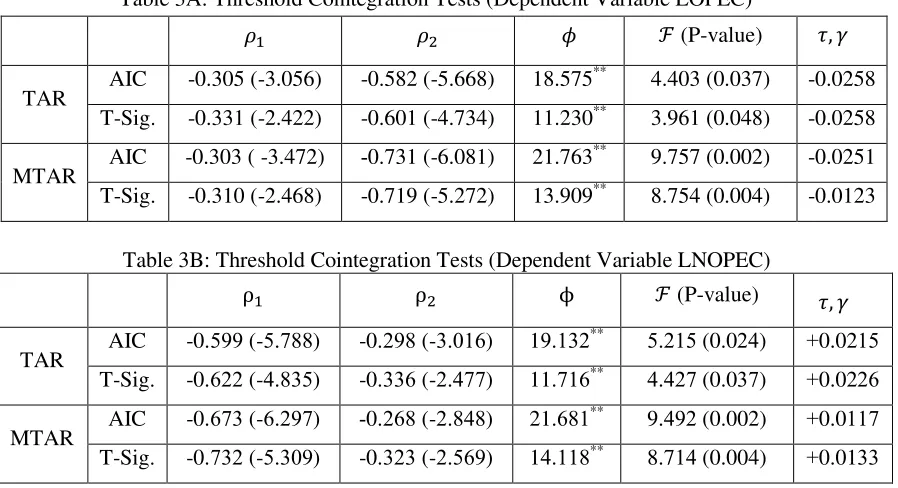
which the lag order is chosen by using the AIC and T-significance tests. Considering the TAR model with
AIC, the point estimates are calculated to be and , and they have the correct
signs for convergence (Table 3A). The statistic is greater than the 1% critical value. It
implies that the null hypothesis of can therefore be soundly rejected, indicating that the series are cointegrated. After confirming cointegration between the oil prices of OPEC and non-OPEC
countries, the null hypothesis of no asymmetry ( ) can be tested by using the standard
13
model following T-significance test for lag selection also completely supports these findings. Therefore,
we can conclude that according to the TAR test, oil prices followed by OPEC and non-OPEC countries
are cointegrated and that the asymmetry is found to exist. The crude oil market prices of OPEC and
non-OPEC have a high asymmetric-cointegration, which may be related to the easy flow of oil market prices
information. The asymmetry feature could be used to stabilize the crude oil prices at an acceptable level
[image:15.612.84.533.231.475.2]from an increase or a decrease in the main place of the crude oil market.
Table 3A: Threshold Cointegration Tests (Dependent Variable LOPEC) iii
Table3B: Threshold Cointegration Tests (Dependent Variable LNOPEC)
Turning to the MTAR and using AIC (Table 3A), the point estimates are found to be
and , which have the correct signs and suggest convergence. The statistic of 21.763
clearly rejects the null hypothesis of no cointegration at 1 % significance level. Given that the value
equals 9.757 with P-value of 0.002, we can reject the null hypothesis of symmetric adjustment. In fact, the
evidence of asymmetric adjustment is further enhanced with the MTAR model. Table 3B also indicates
almost identical results.
Therefore, the asymmetric adjustment is found both in the TAR and MTAR models under the AIC
and T-significance. The point estimates of and are found to be negative, which suggest convergence
in both the TAR and MTAR models. Because , the results exhibit little adjustment for a (P-value)
TAR AIC -0.305 (-3.056) -0.582 (-5.668) 18.575
**
4.403 (0.037) -0.0258
T-Sig. -0.331 (-2.422) -0.601 (-4.734) 11.230** 3.961 (0.048) -0.0258
MTAR AIC -0.303 ( -3.472) -0.731 (-6.081) 21.763
**
9.757 (0.002) -0.0251
T-Sig. -0.310 (-2.468) -0.719 (-5.272) 13.909** 8.754 (0.004) -0.0123
(P-value)
TAR AIC -0.955 (-9.877) -0.857 (-3.610) 15.138
** 9
.819 (0.082) +0.0219
T-Sig. -0.088 (-2.739) -0.330 (-8.288) 11.810** 2.288 (0.038) +0.0280
MTAR AIC -0.083 (-0.858) -0.807 (-8.727) 21.071
**
9.258 (0.002) +0.0118
14
positive and as compared to the substantial decay for a negative and . In other
words, increases are persistent and tend to revert back to the attractor less rapidly, but decreases tend to
revert quickly back to the attractor i.e. long-run equilibrium. Thus, the results show that both the TAR and
MTAR models show that there are asymmetric adjustments in oil prices between OPEC and non-OPEC
countries. Furthermore, it is confirmed from Tables 3A and 3B that the adjustment process is not
persistent toward equilibrium above the threshold for both the TAR and MTAR models. However, the
deviations from equilibrium are almost quickly eliminated when they are below the threshold parameter.
This means that the long-run equilibrium relation below the threshold parameter between the oil price of
OPEC and non-OPEC countries is more stable with an asymmetric adjustment. This asymmetric
adjustment implies some asymmetries between changes in the price of oil for OPEC countries versus the
non-OPEC oil price shocks and vice versa.
3.2 Error correction model
Given the findings of cointegration between the two oil prices, it is possible to estimate the asymmetric
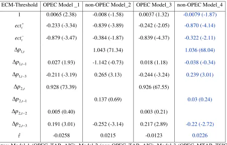
error correction model with the threshold adjustment. The results for the ECM are reported in Table 4.
Interestingly, both the TAR and MTAR models detect asymmetry in the oil price adjustment of OPEC
and non-OPEC countries. The MTAR model, which has a consistent estimate of the threshold, yields the
lowest AIC relative to the other models and the MTAR specification exhibits greater power over the TAR
specification (Enders & Granger 1998). The asymmetric ECM based on the TAR and MTAR
specifications with Eq. (6) and specified errors framework Eq. (7-9) replaces the single symmetric ECM.
Through the comparison between the transitory volatility persistence rate and the permanent
decay rate , the results of the ECM-Threshold-CGARCH model show that the short run volatilities are
less persistent than the long run volatilities. iv
However, these volatilities converge to the mean reversion
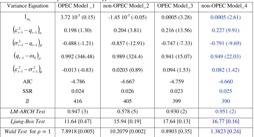
at speed after occurrence of the shocks, because . Thus, would move slowly toward the unconditional variance. This means that the shocks on the long run component do not decay quickly,
15
component (Figures 3) is estimated for the OPEC prices at a high rate of 99.2% using the Student’s
error distributionand 94.1% using Gaussian error distribution (GED).Therefore, these decay rates imply
that approximately 93.8% i.e. of a shock remains even after 8 trading monthsand 61.5%of the shock stays using Student’s and Gaussian error distribution, respectively. For the non-OPEC prices,
the decay rate is also high at 98.9% when we use the GED and 97.8% using normal distribution. Hence
91.5% and 83.7% of the effect of the shocks remains even after 8 months using either the GED and
normal distribution, respectively (Appendix, Figures 2). Using the AIC criterion for the threshold
parameter, even after one year, the shocks on OPEC oil prices persist at 90.8% i.e. , whereas for the non-OPEC oil prices, they are less persistent at 87.6%. By using the T-sig criterion, the results
indicate that even after one year, the shocks on OPEC oil prices persist at 48.2% i.e. , whereas for the non-OPEC oil prices, they are more persistent at 76.6%.
The permanent component coefficients are well-defined for all the models 1-4, implying the slow
convergence of the long-run volatilities to their mean levels, explaining the long-run stability of the
process underlying. In contrast, as the sum of the transitory component parameters is negative for both the
crude oil prices, there is no half-life defined for either the OPEC or non-OPEC oil prices. This result is
due to the high short-run volatility in the transitory variance.
Figures 3a: Conditional and Permanent CGARCH of OPEC and non-OPEC prices
.0000 .0004 .0008 .0012 .0016 .0020 .0024 .0028 .0032
1998 2000 2002 2004 2006 2008 2010
Conditional_CGARCH_Student_lopec_AIC Permanent_CGARCH_Student_lopec_AIC
.000 .001 .002 .003 .004 .005
1998 2000 2002 2004 2006 2008 2010
16
[image:18.612.83.535.360.650.2]Figures 3b: Conditional and Permanent CGARCH of OPEC and non-OPEC prices
Table 4a: ECM-CGARCH Applied to OPEC and non-OPEC Prices 1997.1-2011.4
ECM-Threshold OPEC Model _1 non-OPEC Model_2 OPEC Model_3 non-OPEC Model_4
1 0.0065 (2.38) -0.008 (-1.58) 0.0037 (1.32) -0.0079 (-1.87)
t
ect -0.233 (-3.34) -0.839 (-3.89) -0.242 (-2.05) -0.870 (-4.14)
t
ect -0.879 (-3.47) -0.384 (-1.87) -0.839 (-4.37) -0.322 (-2.11)
t
p1,
1.043 (71.34) 1.036 (68.04)
1 , 1
p t 0.027 (1.93) -1.142 (-0.73) 0.018 (1.18) -0.038 (-0.34)
3 , 1
p t -0.211 (-3.19) 0.265 (3.13) -0.244 (-3.24) 0.239 (3.01)
t
p2,
0.928 (73.39) 0.926 (67.55)
1 , 2
p t 0.137 (0.69) 0.03 (0.24)
2 , 2
p t 0.005 (0.40) 0.003 (0.21)
3 , 2
p t 0.191 (3.01) -0.252 (-3.14) 0.217 (2.89) -0.22 (-2.72)
ˆ -0.0258 0.0215 -0.0123 0.0226
Notes: Model 1 (OPEC_TAR_AIC), Model 2 (non-OPEC_TAR_AIC), Model 3 (OPEC_MTAR_TSIG) and Model 4 (non-OPEC_TAR_TSIG). Using VAR lag selection criteria, we find that the optimal lag is three following the sequential modified LR statistic test, the final prediction error and the AIC. In parentheses, we have the z-statistic.
.000 .001 .002 .003 .004 .005
1998 2000 2002 2004 2006 2008 2010
CONDITIONAL_CGARCH_Gaussian_lopec_TSIG PERMANENT_CGARCH_Gaussian_lopec_TSIG .000 .001 .002 .003 .004 .005 .006
1998 2000 2002 2004 2006 2008 2010
17
Table 4b: Variance Equation CGARCH Applied to OPEC and non-OPEC Prices 1997.1-2011.4
Variance Equation OPEC Model _1 non-OPEC Model_2 OPEC Model_3 non-OPEC Model_4
0
1
3.72 10-5 (0.15) -1.45 10-5 (-0.05) 0.0005 (3.28) 0.0005 (2.61)
1
2
1
tt
q
0.198 (1.30) 0.204 (3.81) 0.216 (13.56) 0.227 (9.91)
1
2
1
t
t q -0.488 (-1.21) -0.857 (-12.91) -0.747 (-7.33) -0.791 (-9.69)
qt1
0
0.992 (346.48) 0.989 (324.4) 0.941 (15.07) 0.949 (22.03)
21
2
1
t
t -0.013 (-0.83) 0.0203 (0.89) 0.094 (1.53) 0.082 (1.42)
AIC -4.786 -4.667 -4.759 -4.660
SSR 0.024 0.026 0.023 0.025
ll
416 405 399 390LM-ARCH Test 0.947 (3) 0.578 (5) 0.930 (2) 0.951 (2)
Ljung-Box Test 11.64 [0.47] 15.94 [0.19] 17.64 [0.13] 16.77 [0.16]
Wald Test for 7.8918 [0.005] 10.2079 [0.002] 0.8903 [0.35] 1.3823 [0.24]
Notes: The z-statistics are in parentheses. The LM-ARCH statistic tests of no ARCH effects in the residuals of the estimated equation, the number of lags is in parentheses. The Ljung-Box statistic tests of no serial correlation in the residuals. The Wald test is running to test the unit value of the persistence parameter using statistic. The p-values are in brackets.
A negative (positive) signals an upward (downward) adjustment of the price startingfrom the next period and from the deviations to the long run equilibrium (Enders & Siklos 2000). A small (high)
value of the long run coefficient indicates that the error correction term of the oil price process is
weakly (strongly) exogenous with respect to the long run relationship between OPEC and non-OPEC
prices. The adjustment of OPEC price process in relation to the positive discrepancies in the long run
equilibrium shows the appropriate negative sign, and the slow adjustment indicates that the OPEC
organization does not prefer modest oil prices. In contrast, a rapid adjustment of non-OPEC price process
in relation to the positive discrepancies in the long run equilibrium signifies a preference of modest oil
prices after they increase. This speed difference between OPEC and non-OPEC price processes is an
evidence of competitive behavior between OPEC and non-OPEC countries. The OPEC producers could
18
assume the OPEC actions, caused the price fluctuations (Hammoudeh 1997). However, our results show
that non-OPEC participants do not follow the OPEC strategies. The asymmetric adjustment provides
evidence that the market participants sometimes misuse their market power in oil price determination.
The point estimates for , i.e., the undervaluation, are in absolute value and are somewhat high
between 0.73 and 0.87 in the model 1 , 3 and 4, suggesting that the deviations between an increase in the
long run and the plausible crude oil prices are eliminated rather quickly. In contrast, the point estimates
for , i.e., the overvaluation, are reported in absolute value and are on the low side between 0.23 and 0.34. In these cases, the asymmetry is largely driven by a strong response to negative shocks. The
negative discrepancies of the OPEC prices from the long run equilibrium are eliminated quite quickly in
comparison to the non-OPEC prices. This result confirms that the non-OPEC countries set modest oil
prices and are more sensible to overvaluation.
Using the T-significance criterion, the results of Models 3 and 4 indicate that there are indeed two
types of asymmetric long run effects: the point estimates for the error correction term are negative for the
OPEC prices, but positive for the non-OPEC prices. Unexpectedly, the LR changes in OPEC crude oil
prices are accompanied by LR changes in non-OPEC prices in the opposite direction. Therefore, when the
crude oil prices tend to be overvalued, an asymmetric phenomenon occurs with an expected negative sign
of , which indicates that OPEC prices will revert to the intrinsic LR equilibrium and therefore have a
stabilizing effect, whilst the non-OPEC has an unexpected positive sign of , which indicates that the
prices will increase, but will revert finally to the LR equilibrium. The result of the non-OPEC price
change can be explained by their excessive aversion behavior.
The non-OPEC (OPEC) prices move upward in the short run, if they are undervalued relative to the
OPEC (non-OPEC) crude oil prices, which would influence the OPEC prices from Model 1 and 3 (Model
2 and 4). The crude oil prices of non-OPEC countries would adjust upwards at a slower rate to correct the
imbalance with the OPEC crude oil prices than would the OPEC prices if they were to adjust upwards to
19
The appearance of imperfect competition, due to many causes, implies an inefficient market. The
subdued adjustment of positive discrepancies to the long run equilibrium may occur because OPEC
countries want to control the high prices of oil and try to sporadically retain the oil prices around
equilibrium level. The non-OPEC countries also provide trivial support in this respect. In the short run,
there is evidence of a causal flow of changes of contemporary oil price from non-OPEC to OPEC
countries and vice versa, with many discernible feedback relationships. The OPEC quota agreements
contribute to this short run price fluctuation. As a result, the price of oil in one group affects the other
group’s price of oil. In particular, the -statistics corresponding to causality reveal that prices of each
group, OPEC and non-OPEC, affect the movements in the other group’s current price rate.
4. Conclusion
The empirical analysis of this paper examined the dynamics of OPEC and non-OPEC oil prices using the
TAR-Error Correction-CGARCH model, which leads to a parsimonious representation of some stylized
features, for the period January 1997 to April 2011. Based on the adjustment rate of the permanent
component errors, the estimated TAR-ECM-CGARCH showed evidence of long run volatility in the
variance and asymmetric effects of negative and positive shocks. Using the AIC criterion for the threshold
parameter, after one year, 90.8% of the effects of the shocks on OPEC oil prices persist, whereas for the
non-OPEC oil prices, less than 87.6% of the effects of the shocks persist. By using the T-significance
criterion, this result indicates that even after one year, the impact of shocks on the OPEC oil prices will
persist at 48.2%, whereas for the non-OPEC oil prices, the impact persists at a higher rate than 76.6%.
These results show that the conditional volatility has a long run memory feature, which supports the long
run memory for oil price volatility.
The slow OPEC adjustment to positive discrepancies in the long run equilibrium shows that OPEC
organization does not prefer modest oil prices, while a rapid adjustment in the non-OPEC process
20
OPEC and non-OPEC price adjustments imply that there is evidence of a competitive behavior and
different profit and pricing strategies between OPEC and non-OPEC countries. The OPEC producers
could not drive down (up) crude oil market prices. Market traders and speculators, who assume the OPEC
actions, cause the price fluctuations. Additionally, our results show that the non-OPEC participants do not
follow the OPEC strategies. In other words, this implies that OPEC is not the leader in the world crude oil
market. The future work has to use the asymmetric multivariate GARCH models to better understand the
permanent and transitory components in the crude oil market prices.
References
1. Adelman, MA., 1962. Natural Gas and the World Petroleum Market. The Journal of Industrial
Economics 10, 76-112.
2. Alexander C. and E. Lazar, 2006. Normal Mixture GARCH(1,1): Applications to exchange rate
modeling. Journal of Applied Econometrics 21: 307 – 336. DOI: 10.1002/jae.849.
3. Angrist, J., Graddy, K. and Imbens, GW., 2000. The Interpretation of Instrumental Variables
Estimators in Simultaneous Equations Models with an Application to the Demand for Fish. The
Review of Economic Studies 67 (3), 499-527.
4. Balke, NS., Brown, SPA., Yucel, MK., 1998. Gasoline and crude oil prices: an asymmetric
relationship? Federal Reserve Bank of Dallas Economic Review, First Quarter, 2–11.
5. Berndt, ER., and Wood, DO., 1975. Technology, prices, and the derived demand for energy. The
Review of Economics and Statistics 57(3), 259—268.
6. Bekiros, SD., and Diks CGH., 2008. The relationship between crude oil spot and futures prices:
Cointegration, linear and nonlinear causality. Energy Economics 30(5), 2673-2685.
7. Bollerslev T. and R.F. Engle, 1993. Common Persistence in Conditional Variances. Econometrica 61,
166-187.
8. Borenstein, S., Cameron, AC., Gilbert, R., 1997. Do gasoline prices respond asymmetrically to crude
oil price changes? Quarterly Journal of Economics 112, 305–339.
9. Chan , KS., 1993. Consistency and limiting distributions of the least Squares estimator of a Threshold
Autoregressive Model. The Annals of Statistics 21, 520-533.
10. Chen, Li-Hsueh, T., Miles Finney, Lai, Kon S., 2005. A threshold cointegration analysis of
21
11. De Santis, RA., 2003. Crude oil price fluctuations and Saudi Arabia's behavior. Energy Economics
25(2), 155-173.
12.
Diebold F.X. and J.A. Lopez,
1995
. Modeling Volatility Dynamics.
Macro-econometrics,
Recent Economic Thought
Series Volume 46:427-472.
13. Enders, W., Granger C., 1998. Unit root tests and asymmetric test with an example using the term
structure of interest rate, Journal of Business and Economic Statistics 16, 304-311.
14. Enders, W., Siklos, PL., 2001. Cointegration and threshold adjustment. Journal of Business and
Economic Statistics 19, 166–176.
15. Energy Information Administration (EIA), 1999. Prices Changes in the Gasoline Market: Are
Midwestern gasoline prices downward sticky? US Department of Energy, Washington, DC.
16. Engle R.F. and A.J. Patton, 2000. What good is a volatility model? Quantitative Finance 1(2), 237–
245.
17. Engle, R. and G. Lee, 1999. A Long-Run and Short-Run Component Model of Stock Return
Volatility, in Cointegration, Causality and Forecasting. Edited by R. Engle and H. White, Oxford
University Press.
18. Engle R.F. and G. Gonzalez-Rivera, 1991. Semi-parametric ARCH Models. Journal of Business &
Economic Statistics 9(4): 345-359.
19. Engle, R. and Granger, C.W.J. 1987. “Co-integration and error-correction: Representation, estimation, and testing.” Econometrica 35: 315-329.
20. Ewing, B., Hammoudeh, S and Thompson, 2006. Examining Asymmetric Behavior in US Petroleum
Futures and Spot Prices. The Energy Journal 27(3), 9-23.
21. Gately, D., 1984. A ten-year retrospective: OPEC and the world oil market. Journal of Economic
Literature 22(3), 1100—1114.
22. Gately, D., 1993. The Imperfect Price-reversibility of World Oil Demand. The Energy Journal 14(4),
163-182.
23. Gately, D., and Huntington, HG., 2002. The Asymmetric Effects of Changes in Price and Income on
Energy and Oil Demand. The Energy Journal 23 (1), 19-55.
24. Godby, R., Lintner, AM., Stengos, T., Wandschneider, B., 2000. Testing for Asymmetric Pricing in
the Canadian Retail Gasoline Market. Energy Economics 22, 349–368.
25. Goldberger, AS., 1991. A course in econometrics. Harvard University Press, Cambridge, MA.
26. Gospodinov, N., 2008. Asymptotic and bootstrap tests for linearity in a TAR-GARCH(1,1) model
with a unit root. Journal of Econometrics 146(1), 146-161.
27. Griffin, JM., 1985. OPEC behavior: A test of alternative hypotheses. The American Economic Review
22
28. Hamilton, JD., 2008. Understanding Crude Oil Prices. National Bureau of Economic Research,
Working Paper number 14492.
29. Hammoudeh, S., 1997. Oil Pricing Policies in a Target Zone Model. Research in Human Capital and
Development, Vol. 11-B: 497-513.
30. Hammoudeh, S., Chen, LH., and Fattouh B., 2010. Asymmetric Adjustments in Oil and Metals
Markets. The Energy Journal 31(4): 183-203.
31. Hatanaka M., 1996. Time-Series-Based Econometrics: Unit Roots and Co-integrations (Advanced
Texts in Econometrics). Oxford University Press. Reprinted 2003. ISBN-13: 978-0198773535.
32. Hausman, JA., 1975. Project independence report: an appraisal of U.S. energy needs up to 1985. The
Bell Journal of Economics 6 (2), 517-551.
33. Holton, Glyn A., 2014. Value-at-Risk: Theory and Practice, 2nd ed. e-book at http://value-at-risk.net.
34. Horvath & Watson, 1995. Testing for Cointegration when some of the Cointegrating Vectors are
Pre-specified. Econometric Theory 11, 984-1014.
35. Jones, Clifton T., 1990. OPEC Behavior under Falling Prices: Implications for Cartel Stability, The
Energy Journal 11(3), 117-130.
36. Kang, SH., Kang, SM., and Yoon SM., 2009. Forecasting volatility of crude oil markets. Energy
Economics 31(1), 119-125.
37. Kennedy, M., 1974. An Economic Model of the World Oil Market. The Bell Journal of Economics
and Management 5 (2), 540-577.
38. Lin, CYC., 2009. An Empirical Dynamic Model of OPEC and non-OPEC. Presented in International
Association for Energy Economics North American conference, Houston, September.
39. Li., Raymond, 2010. The Role of OPEC in the World Oil Market. International Journal of Business
and Economics 9, (1), 83-85.
40. Manski, CF., 1995. Identification Problems in the Social Sciences. Harvard University Press,
Cambridge, MA.
41. Mohammadi, H., and Su, L., 2010. International evidence on crude oil price dynamics: Applications
of ARIMA-GARCH models. Energy Economics 32(5), 1001-1008.
42. Ng, S., Perron, P., 2001. Lag Length Selection and the Construction of Unit Root Test with Good
Size and Power. Econometrica 69, 1519-1554.
43. Nordhaus, WD., 1980. Oil and Economic Performance in Industrial Countries. Brookings Papers on
Economic Activity 2, 341-399.
44. Perron, P., Rodriguez, G., 2001.Residual based tests for cointegration with GLS detrended data,
23
45. Petrucelli, J. and S. Woolford (1984). A Threshold AR(1) Model. Journal of Applied
Probability 21, 270 - 86.
46. Poon S.H., Hyung, N. and C.W.J. Granger, 2006. A Source of Long Memory in Volatility. Available
at SSRN: http://ssrn.com/abstract=904582 or http://dx.doi.org/10.2139/ssrn.904582.
47. Ray, BK. and RS. Tsay, 2000. Long-range dependence in daily stock volatilities. Journal of Business
& Economic Statistics 18: 254–262.
48. Stock J.H. and M.W. Watson, 1988. Testing for Common Trends. Journal of the American Statistical
Association 83(404), 1097-1107.
24 Appendices
Figures 1: OPEC and non-OPEC prices
Figures 2: Persistence shocks over month’s horizon on OPEC and non-OPEC prices
2.0 2.5 3.0 3.5 4.0 4.5 5.0
1998 2000 2002 2004 2006 2008 2010
Logarithmic price of OPEC
2.0 2.5 3.0 3.5 4.0 4.5 5.0
1998 2000 2002 2004 2006 2008 2010
Logarithm price of Non OPEC
-.5 -.4 -.3 -.2 -.1 .0 .1 .2 .3 .4
1998 2000 2002 2004 2006 2008 2010
First difference of Logarithm price of OPEC
-.5 -.4 -.3 -.2 -.1 .0 .1 .2 .3 .4
1998 2000 2002 2004 2006 2008 2010
First difference of Logarithm price of Non OPEC
0.0 0.1 0.2 0.3 0.4 0.5 0.6 0.7 0.8 0.9 1.0
4 12 20 28 36 44 52 60
OPEC_TSIG NOPEC_TSIG 0.0 0.1 0.2 0.3 0.4 0.5 0.6 0.7 0.8 0.9 1.0
4 12 20 28 36 44 52 60
25
Table A: World Oil Supply and Demand Barrels (Per Million Day)
Year 2005 2006 2007 2008 2009
OPEC Supply to World market 34.7 35.4 34.6 35.6 33.3 non-OPEC Excess Demand-Supply 34.1 34.6 35.6 35.1 33.0 Source: Oil Market Report, Annual Statistical Supplement, I.E.A. 2010
Table B: World Oil Production: OPEC and non-OPEC (%)
Year 2005 2006 2007 2008 2009
OPEC 40.50 40.20 41.98 41.25 39.32 non-OPEC 59.50 59.80 58.02 58.75 60.68 Source: Annual Report, S.A.M.A. 2010
End Notes:
i
As demonstrated by Sichel (1993), a negative “deepness” (i.e. ) of implies that increases tend to persist, whereas decreases tend to revert quickly towards equilibrium.
iiIn the EG’s test: one sided (lower tail) test of the null hypothesis that the variables are not co integrated; at the 1, 5, and 10 per cent level critical value equal -4.02, -3.40 and -3.09, respectively (Rapach & Weber 2004). In the PR’s test: one sided (lower-tail) test of the null hypothesis that the variables are not co-integrated; at the 1, 5, and 10 per cent level critical value equal -3.33, -2.76 and -2.47, respectively (Perron & Rodriguez 2001).
iii
The double * indicates significance-level at 1%. The values corresponding to are compared with tables computed by Enders and Siklos (2001). The numbers in parentheses in the third and fourth columns denote t-values.
iv