An ANN based Two Pass-Two Phase Adaptive Filtering
of a Digital Image Corrupted by SPN
Prakash Ch. Dash
1, Manoj Kumar Mishra
2, Nachiketa Tarasia
2, Sarita Das
3, G. B. Mund
2MITM1, KIIT University2, EAST3 Bhubaneswar, Orissa, India
ABSTRACT
Images get contaminated due to different noises at various stages of processing and Salt and Pepper is one such noise. The noise removal approach used for filtering mainly differs in their basic methodologies, but the purpose is to suppress different types and percentage of noise. Some of the filtering schemes replace those corrupted pixels by indentifying the positions of the corrupted pixels in the observed noisy image, with the help of a noise detector, whereas others remove all the pixels irrespective of corruption. This paper investigates the former method in denoising a digital image through incorporation of an adaptive threshold into the noise detection process. The adaptive threshold value thus obtained is based on the noisy image characteristics and their statistics using LeNN (Legendre Neural Network) and the patterns of input image are taken to train FLANN (Functional Link Artificial Neural Network) corrupted by SPN(Salt & Pepper noise). Comparative analysis on standard images at different noise percentage shows that the proposed scheme outperforms the existing schemes in terms of PSNR (peak signal to noise ratio). Thus, the proposed method named as “Two pass- Two phase adaptive filtering mechanism” is feasible and also makes it an efficient filter to restore the gray image fairly well preserving the quality of the filtered image, and also provides a better visual perception.
General Terms
Neural network, Image, NoiseKeywords
MLP, FLANN, LeNN, Salt & Pepper noise.
1.
INTRODUCTION
In this era of information technology, processing visual information through computer has become a necessity, as vision allows human beings to perceive and understand the world around them in a better manner. That encourages the researchers around the world to put significant effort to work in the field of digital image processing. Digital image filtering is one important research area in the field of image processing, since original images may be degraded by various means and noise types. SPN (Salt & Pepper noise) is one such noise in a digital image caused by noisy sensors and faulty hardware at the time of transmission through a nonlinear channel, acquisition, and storage. Manual detection and removal of such noises from a digital image by any human expert is not an easy task. Therefore, developing an efficient noise removal mechanism is the motivation behind this work.
In a noisy image, it is observed that number of pixels corrupted is not equal to total number of pixels in an image. Therefore, probability of corruption is less than 1 in a corrupted image. Hence, it is assumed that a corrupted pixel is
surrounded by some of the non-noisy pixels or healthy pixels. It is noteworthy to mention that the above assumption holds as long as the percentage of noise is very less. But this assumption does not hold if the noise percentage is very high. Usually filtering is either performed upon all pixels irrespective of corruption or by detecting the noisy the pixels and replacing them with a good one. The former one is unnecessary and time consuming method to perform filtering operation on all the pixels to eliminate the noise. But the latter approach is efficient and useful because filtering operation is carried out only upon those corrupted pixels. It is also computationally economical to filter only the corrupted pixels and not to change the healthy pixels. Moreover, applying filter operation upon all the pixels irrespective of corruption causes blurring effect on the restored image. Therefore, the filtering scheme should indentify the positions of the corrupted pixels in the observed noisy image with the help of a noise detector. Then the noisy pixels are replaced by good pixels. Thus, detection based noise removal approach saves unnecessary time consumption, thereby reducing the blurring effect of restored image.
Most of the filter parameters depend on the level and type of corruption. Some of the traditional reported filtering methodology for image restoration is based on the linear processing of image. The performance and quality of restored image described in Moving Average [1], Median (3 × 3) and Median (5 × 5) [2] is very poor because it acts like a low pass filter which blocks all high frequency components of the image like edges and noise, thus blurs the image. In WM for k = 1, k = 2, the filters work better when the noise percentage is low but beyond 10% of noise the performance starts deteriorating. If noise appears as blotch in a window, it leaves the blotch as it is as if no filtering is done [11-14].
Researchers have also conducted some research works in detection based linear filtering. Progressive-Switching Median [2] presents a very good filter for fixed valued impulsive noise but for random values the performance is abysmal. Another scheme described in Peak and Valley [4] is computationally efficient over others but at the same time it spoils non-noisy pixels to a greater extent. The performance of Advanced Impulse Detection Based on Pixel-Wise MAD [15] is more than average but fails when the edge density is more. Differential Ranked Impulse Detector [3] is a good filter in low noise conditions but the performance starts degrading beyond 20% of noise. It also leaves noise blotch without correcting. The performance of Enhanced Ranked Impulse Detector [3] is very good at low noise but fails miserably at noise density more than 20%.
adapt themselves to the changing conditions of noise. In such an application, the image filter must adapt the image local statistics, the noise type and adjust itself to changing characteristics so that the overall filtering improves substantially. Soft computing methodologies particularly ANNs are used in image processing because they mimic the human capability of making decision in ambiguous environment. So, the application of artificial neural network techniques in image processing can be adaptive and adjust itself in changing environment through training its neurons accordingly. So, this paper has taken the help of ANN to design an adaptive filter to detect the SPN. The image filtration must be adaptive towards the change of local statistics, noise type and percentage of noise added, so that the quality of restored image is better than others. Thus the paper presents “a two pass-two phase adaptive filtering of a digital image corrupted by SPN”. The proposed image filter efficiently removes noise of a digital image up to 30%.
The rest of the paper is organized as follows. Section 2 mainly recollects some of the previously reported image filtering schemes and their characteristics. Section 3 proposes a model to remove SPN noise using ANN. Details of simulation and comparative results are described in Section 4. Section 5 provides concluding remark, with scope for further research work. References are listed in the last section.
2.
RELATED WORK
Neural networks have already been applied in several domains of image processing including image filtering. ANN has the powerful learning techniques that adapt itself in a highly nonlinear environment [5] and gives better approximation to the nonlinear function. It has also the ability of taking decision in ambiguous, uncertain and changing environment (i.e. the type of image, characteristic and density of noise). So, the advantages of ANN model are: (i) its ability to learn based on optimization technique of an appropriate error function, and (ii) excellent performance for approximation of nonlinear functions.
MLP is a type of ANN which consists of multiple layers i.e. with one or more hidden layer(s) between its inputs and outputs and uses back propagation algorithm for the training of NN. A pattern is applied to the input layer, but no computations takes place in this layer. Thus, the output of the nodes of this layer is the input pattern itself. All the nodes in each layer (except the input layer) of the MLP contain a nonlinear tanh() function. The weighted sum of outputs of a lower layer is passed through the nonlinear function of a node in the upper layer to produce its output. The outputs of the final layer (output layer) are compared with a target pattern associated with the input pattern. The error between the target pattern and the output layer node is used to update the weights of the network. The mean square error (MSE) is used as a cost function. Due to the multilayer architecture, the MLPs are inherently computationally intensive. Although the MLP is widely used due to robust solution and effective filtering, its excessive training time and high computational complexity appear as two major drawbacks of this approach. RBFN is another type of Neural Network that works as alternative of MLP. The Gaussian function is used as nonlinear function in RBFN [7]. The functional link artificial neural network (FLANN) by Pao [6] can be used for function approximation and pattern classification with faster convergence and lesser computational complexity than a MLP network. The computational time is less due to absence of hidden layer in this type of network. A FLANN can be trained using trigonometric, exponential, and polynomial functions for
functional expansion as reported [8], [9]. But practically, large training time of FLANN makes it unattractive for implementation. Legendre Neural Network (LeNN) is another advance neural network which is very similar to FLANN but Legendre polynomial functions are used in LeNN instead of trigonometric and exponential function as in FLANN. The Legendre polynomial Function has faster training convergence than FLANN [10]. By analyzing the above facts, the study motivates to work further towards improving and developing an efficient detector for identification of noisy pixels and devising an adaptive thresholding mechanism that will make the detection process more accurate.
Therefore, the proposed method uses LeNN for the calculation of threshold values which is very important for detection of noisy pixels. The importance of the work is that adaptive threshold values are obtained for each 3×3 window, which is used to indentify black and white spots that would make the noise detection more reliable for effective suppression of noises and fairly restoring the image. Most of the previously discussed filtering methodology has some drawbacks due to which they are unable to produce the image close to original. The traditional filtering mechanisms suffer from so many drawbacks like over filtering, distortion, blurring, high computational complexity etc. The next section describes the detection and filtration mechanism of the proposed scheme.
3.
PROPOSED SCHEME
The proposed scheme as shown in figure 1, applies an adaptive detection based filtering mechanism to maintain the image details. Sub-sections „3.2‟, „3.3‟, „3.4‟, „3.5‟ and „3.6‟ describe the sequence of the proposed method. A generic mathematical model for degraded image is described in subsection „3.1‟, given below.
3.1
Salt & Pepper Noise (SPN)
A two-dimensional Matrix is used to store the values of a digital image. Any changes in values of the matrix cause noise in the image.
i
j
Y
i
j
N
i
j
X
,
,
,
...……….(1)Where Y represents the original image, X represents the observed degraded image and N is the value of the noise added with a probability p. A pixel value at location (i, j) of image is said to be not corrupted if the value of N is 0 with a probability 1- p. Therefore, an image corrupted with Salt & Pepper Noise (SPN) or alternatively known as Fixed Valued Impulsive Noise may formally be defined as:
Let Y(i, j) be any gray level value lies between a min and max value of an original image Y at pixel location (i, j). Similarly, let X(i, j) be the gray level of the noisy image X at pixel location (i, j). So,
p y probabilit with j i N j i Y p y probabilit a with j i Y j i X , , 1 ,, ...
(2)
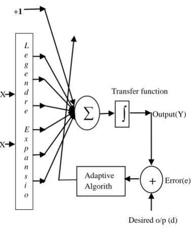
Figure 1: Block diagram of proposed adaptive filtering scheme
3.2
Training of FLANN
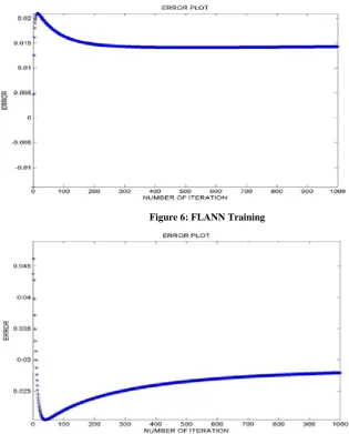
The proposed technique initially takes a corrupted image with some known percentage of SPN and then the input patterns of this noisy image (i.e. moving window of size of 3×3) are taken to train FLANN. The target will be the corresponding middle pixel of the selected window from original image. This process continues iteratively till all pattern of the image gets completed. The whole process is performed for required number of times till error is minimized as depicted in figure 2. The training convergence characteristics of the network are shown in Figure 6. For functional expansion of the input pattern, care has been taken to choose appropriate trigonometric functions.
Figure 2: Pixel training of FLANN
This process is followed by threshold training, threshold calculation, noise detection and filtering mechanism. The threshold value of each test window is obtained based on the noisy image characteristics and their statistics using LeNN. Noise detection is done by comparing the threshold value with another value called „decision factor‟. Median filtering is performed selectively based on the result of this comparison.
3.3
Adaptive Threshold training and its
calculation using LeNN
[image:3.595.54.278.375.732.2]As discussed above in section II, the advantages of using the LeNN (to find threshold) over other ANNs is lesser number of computation. Back propagation algorithm is used for learning of LeNN and also the network has lesser computational load and faster convergence rate than multilayer and FLANN. The Structure of LeNN is shown figure 3.
Figure 3: Structure of LeNN
The detector formed by LeNN after the training is very simple and efficient, which takes the mean (µ) and variance (σ2) of a moving window of size 3 × 3 as input. Here, the computational formula is used for variance (σ2
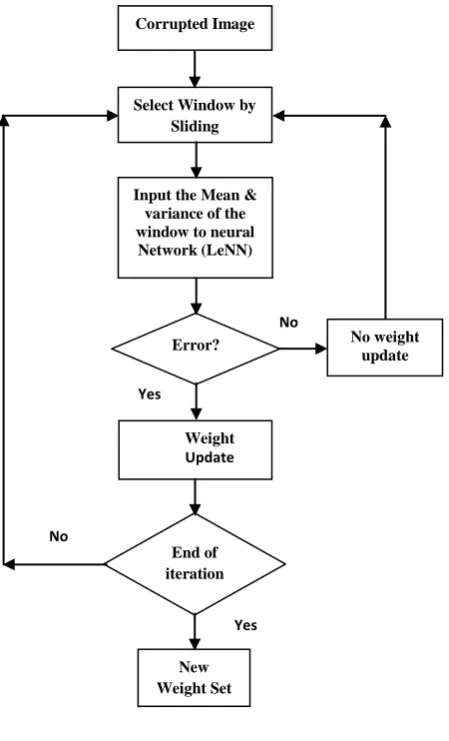
). In order to calculate the error, the actual output on the output layer is compared with the desired output. Depending on this error value, the weight matrix between the input and output layers is updated using back propagation learning algorithm. The Flow chart of threshold training and training convergence characteristics of the network are shown in figure 4 and Figure 7 respectively. Testing the correctness of a pixel is
Yes No
Corrupted Image Detection of SPN at Center Pixel Selection of Window by Sliding Signal to choose new window
Recursive Median Filtering Replacement of corrupted
pixel Filtered image Corrupted Image
Yes
No
End of iteration
New Weight Set No
Yes Weight Update
Error? No weight update Input the pixels
of window to Neural Network
(FLANN) Corrupted Image
Select Window by Sliding
X 2 X 1
L e g e n d r e
E x p a n s i o n
Output(Y) Transfer function
Error(e) Adaptive
Algorith m
+
+
∑
∫
+1
[image:3.595.330.521.405.633.2]solely dependent on the threshold value for that window. Each window of the image has different mean (µ) and variance (σ2) values. So the threshold value obtained is different for each window according to the window characteristics and their statistics, due to which the threshold value is adaptive in nature and able to detect the corrupted pixel at different noise density. Equation-3 denotes the recursive formula to generate Legendre polynomials for LeNN expansion [10].
Figure 4: Threshold training
n
xL
x
nL
x
n
x
L
n 12
1
n n 11
1
...(3)Computational formula for variance is given by
nM i N j ij
n
X
11
2 2
2
..…..(4)Where,
µ=mean(X W)
X W = pixels of the selected window of size 3×3 n=Number of pixels in a window
σ2
=Variance
3.4
Detection and filtration of SPN noise
The optimal performance and efficiency of the filtering scheme lies on the accuracy and robustness of noise detection mechanism. The methodology used here to detect corrupted pixels and their removal is very simple, efficient, and depends upon the feature of neighborhood pixel characteristics. The proposed filtering scheme works in Two Pass- Two Phase method. Each pass goes through phase1 i.e. detection and immediately followed by phase 2 i.e. filtration. First phase is to identify the corrupted pixels and second phase is to replace the corrupted pixels with a good pixel. First pass detects to remove the white spots by comparing the threshold value Th1with a decision factor D1. While, second pass detects to
remove the black spots by comparing the threshold value Th2
with another decision factor D2 for the same window. It can
be noted that 1st pass is performed recursively from top left to bottom-right corner of the noisy image by moving the test window row wise. The partial filtered image obtained after the 1st pass is then subjected to 2nd pass of the algorithm, where salt & pepper noise are detected in vertical fashion i.e. column wise. Removal of the corrupted pixels is performed by Median filtering and the Median filtering is performed selectively and recursively to remove corrupted pixels, based on the result of this comparison.
3.5
Recursive Filtering mechanism
In pass1 and pass2, the middle pixel of a sliding (3 × 3) window of the image matrix is considered to be corrupt and checked for fitness by applying LeNN detection algorithm. If it is found to be corrupt, then it is immediately filtered out i.e. replaced by median value of that window. Similarly, in the next adjacent window, the fitness of the middle pixel is tested by considering the gray level of the already filtered pixel rather than that of the original one. In this fashion, median filtering is carried out recursively by replacing only at the location of the faulty pixel as opposed to the conventional median filter. Mathematically,
i
,
j
median
X
if
N
i
,
j
0
X
w...………(5)
3.6
Two Pass-Two Phase Adaptive
Filtering Algorithm
The proposed mechanism is partitioned into two procedures namely pass1 and pass2. Each pass goes through phase1 and immediately followed by phase2. Threshold computation and noise detection are incorporated into phase1 and phase 2 involves replacement of the corrupted pixel with median value of that window. The algorithms for pass1 and pass 2 are given below.
Pass 1: Threshold calculation, noise detection and partial filtration
Input: Noisy image
Step 1: Select a test window X W of size 3 × 3 located at the top-left corner of the observed image X.
XW =
Step 2: Compute the values of xk „s for k= 1….8 as follows:
x1=( Xi−1,j−1 +Xi+1,j+1)/2-Xi,j
x2=( Xi+1,j−1 + Xi-1,j+1 )/2-Xi,j
1 j 1, i j 1, i 1 -j 1, i 1 j i, j i, 1 -j i, 1 j 1, -i j 1, -i 1 -j 1, -iX
X
X
X
X
X
X
X
X
Yes No End of iteration New Weight Set No Yes Weight UpdateError? No weight update Input the Mean &
variance of the window to neural Network (LeNN) Corrupted Image
Cameraman.tif (Original image)
Cameraman.tif 15% noisy
x3=( Xi-1,j+ Xi+1,j)/2-Xi,j
x4=( Xi,j-1 + Xi,j+1)/2-Xi,j
x5=( Xi-1,j-1 + Xi-1,j+1)/2-Xi,j
x6=( Xi-1,j+1 + Xi+1,j+1)/2-Xi,j
x7=( Xi+1,j−1 + Xi+1,j+1)/2-Xi,j
x8=( Xi+1,j-1 + Xi-1,j-1)/2-Xi,j
Step 3: Input the values of x1, x2…………x8 to the functional link neural network (FLANN). Functionally expand it as discussed above in subsection-B that produces an output known as decision factor D1(i, j)
Step 4: Calculate a threshold value Th1 as described in subsection-C given above.
Step 5: If D1(i, j) > Th1 then the test pixel X(i, j) is corrupted
Else the test pixel X(i, j) is not corrupted (subsection-D)
Step 6: If corrupted, median filtering is performed at location (i, j) by replacing X(i, j) pixel as mentioned in subsection-E.
Step 7: Repeat the above mentioned steps for each test window from top left to bottom-right corner of the noisy image by moving the window row wise.
Output: Partial filtered image
Pass 2: Threshold calculation, noise detection and complete filtration
Input: Partial filtered image
Step 1: Select a test window X W of size 3 × 3 located at the top-left corner of the partial filtered image X obtained from pass one.
Step 2: Compute the values of xi „s for i= 1….9 as follows:
x1= ( Xi−1,j−1 +Xi+1,j+1)/2-Xi,j
x2= ( Xi+1,j−1 + Xi-1,j+1 )/2-Xi,j
x3= ( Xi-1,j+ Xi+1,j)/2-Xi,j
x4= ( Xi,j-1 + Xi,j+1)/2-Xi,j
x5= ( Xi-1,j-1 + Xi-1,j+1)/2-Xi,j
x6= ( Xi-1,j+1 + Xi+1,j+1)/2-Xi,j
x7= (Xi+1,j−1 + Xi+1,j+1)/2-Xi,j
x8= (Xi+1,j-1 + Xi-1,j-1)/2-Xi,j
x9= (Xi−1,j−1+Xi−1,j +Xi−1,j+1+ Xi,j−1+Xi,j+Xi,j+1 +
Xi+1,j−1+Xi+1,j+Xi+1,j+1)/9- Xi,j
Step 3: Input the values of x1, x2…………x9 to the functional link neural network(FLANN), Functionally expand it as discussed in subsection-B that produces an output known as decision factor D2(i, j)
Step 4: Calculate a threshold value Th1 as described in subsection-3.3 given above.
Step 5: If D2 (i, j) > Th2 the test pixel X(i, j) is corrupted Else the test pixel X(i, j) is not corrupted (subsection-D)
Step 6: If corrupted, median filtering is performed at location (i, j) by replacing X(i, j) pixel as mentioned in subsection-E.
Step 7: Repeat the above mentioned steps for each test window from top left to bottom-right corner of the partial filtered image by moving the window column wise.
Output: Complete filtered image
4.
SIMULATION AND EXPERIMENTAL
STUDIES
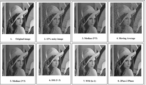
In this proposed work, simulations are carried out with MatLab ver7.9, Pentium dual core processor, 1.6 GHz, and 512MB RAM. Here the images used for simulations are ‟cameraman‟ and ‟lena‟ as shown in fig. 4 and 7 respectively, which are standard grayscale images of size 256×256 and 512×512. The image “Cameraman” is corrupted with 15% SPN before filtration and is subjected to training using FLANN for 1000 iterations. Similarly, the threshold training process is carried out using LeNN for 1000 iterations. The convergence characteristics of FLANN and LeNN are shown in figure 6 and 7. The initial weights have been taken within the range of -0.5 to +0.5 and randomly distributed between layers. The bias and learning rate are set to 1.0 and 0.001. It can be noted that once neural network is trained with an image corrupted by SPN, it can be applied to filter any kind of image corrupted with Salt and Pepper noise. Therefore, it is applied to test „lena‟ image after training. The performance of a method can be judged by peak-signal-to-noise ratio (PSNR) in dB, as given in equation (6) i.e. the noise removal capability of the proposed scheme with existing schemes and subjective evaluation i.e. from seeing the image after filtration. PSNRout and subjective evaluation are shown in table 1 and figure 8 respectively. Experiments were performed to evaluate the performance of the proposed filter by comparing with Median (3×3) [2], Median (5×5) [2], and Moving Average [1], SM (5×5) [16], WM (k=1)[11-14]
j i
j i j i
x
r
MN
PNSR
,
2 , ,
2
10
1
255
log
[image:5.595.312.544.432.628.2]10
………….(6)Figure 5: FLANN is trained with Cameraman.tif
5.
CONCLUSION
denoising scheme achieves better performance that is apparent from the visual differences and also the improvement in PSNR. Development of parallel algorithms can also be done for additional reduction in computational overhead.
Figure 6: FLANN Training
[image:6.595.74.523.566.783.2]Figure 7: Convergence graph of Threshold Training of LeNN at 15 %
Table 1: PSNRout (dB) of Lena image corrupted by SPN at different noise
Filter Type
Noise Percentage
5%
10%
15%
20%
25%
30%
Median(3*3)
33.6860
32.4224
31.5091
30.5041
29.3601
28.2508
Median(5*5)
29.5180
28.2036
27.8800
26.5658
25.8428
25.1408
Moving average
27.0811
24.2884
22.5301
21.0807
20.9156
19.8237
Weighted Median 35.1084
31.2634
27.8217
25.5039
23.6125
22.1492
Switching Median 35.9021
32.2965
31.4237
29.3126
28.2845
26.1026
Figure 8: Subjective Evaluation
Figure 9: PSNR (dB) variations of Lena image corrupted with SPN
2. 15% noisy image
1. Original image 3. Median (5*5) 4. Moving Average
6. SM (5×5)
[image:7.595.143.444.453.643.2]6.
REFERENCES
[1] R. C. Gonzalez and R. E. Woods. Digital Image Processing. Addison Wesley, 2nd edition, 1992. [2] Z. Wang and D. Zhang. Progressive Switching Median
Filter for the Removal of Impulse Noise from Highly Corrupted Images. IEEE Transactions on Circuits and Systems–II: Analog and Digital Signal Processing, 46(1):78 – 80, January 1999.
[3] C. Butakoff and I. Aizenberg. Effective Impulse Detector Based on Rank-Order Criteria. IEEE Signal Processing Letters, 11(3):363 – 366, March 2004.
[4] P. S. Windyga. Fast Impulsive Noise Removal. IEEE Transactions on Image Processing, 10(1):173 – 179, January 2001.
[5] S. Haykin., Neural Networks, Ottawa.ON.Canda, Maxwell Macmillan, 1994.
[6] Y.H .Pao, Adaptive Pattern Recognition and neural networks. Reading .MA addison- Wesley.1989.
[7] J. Park, and I. W. Sandberg, “Universal approximation using radial basis function networks, ”Neural Comput., vol. 3, 1991,pp. 246–257.
[8] J. C. Patra, R. N. Paul, B. N. Chatterji, G. Panda, Identification of nonlinear dynamic systems using functional link artificial neural networks, IEEE Trans., Systems, Man and Cybernetics, Part B, Vol.29, April 1999, pp.254-262.
[9] Chebysev Functional Link Artificial Neural Networks for Denoising of Image Corrupted by Salt and Pepper Noise , ACEEE International Journal on Signal and Image Processing Vol 1, No. 1, Jan 2010.
[10] Nonlinear channel equalization for wireless communication systems using Legendre neural networks Jagdish C. Patra, Pramod K.Meher, Goutam Chakraborty, Elsevier, Signal Processing 89 (2009) 2251–2262.
[11] S. J. Ko and Y. H. Lee. Center Weighted Median Filters and Their Applications to Image Enhancement. IEEE Transactions on Circuits and Systems, 38(9):984 – 993, September 1991.
[12] T. Chen and H. R. Wu. Adaptive Impulse Detection Using Center-Weighted Median Filters. IEEE Signal Processing Letters, 8(1):1 – 3, January 2001.
[13] D. R. K. Brownrigg. The Weighted Median Filter. Communications ACM, 27:807 – 818, August 1984. 75. [14] B. I. Justusson. Median Filtering: Statistical Properties.
Two-Dimensional Signal Processing-II, T. S. Hwang Ed. New York: Springer Verlag, 1981.
[15] V. Crnojevic, V. Senk, and Z. Trpovski. Advanced Impulse Detection Based on Pixel-Wise MAD. IEEE Signal Processing Letters, 11(7):589 – 592, July 2004.