A Budyko framework for estimating how spatial heterogeneity and lateral moisture redistribution affect average evapotranspiration rates as seen from the atmosphere

www.hydrol-earth-syst-sci.net/21/217/2017/ doi:10.5194/hess-21-217-2017

© Author(s) 2017. CC Attribution 3.0 License.

A Budyko framework for estimating how spatial heterogeneity and

lateral moisture redistribution affect average evapotranspiration

rates as seen from the atmosphere

Elham Rouholahnejad Freund1and James W. Kirchner1,2,3

1_{Department of Environmental Systems Science, ETH Zurich, 8092 Zürich, Switzerland} 2_{Swiss Federal Research Institute WSL, 8903 Birmensdorf, Switzerland}

3_{Dept. of Earth and Planetary Science, University of California, Berkeley, CA 94720, USA}

Correspondence to:Elham Rouholahnejad Freund ([email protected]) Received: 18 August 2016 – Published in Hydrol. Earth Syst. Sci. Discuss.: 31 August 2016 Revised: 16 November 2016 – Accepted: 17 November 2016 – Published: 11 January 2017

Abstract. Most Earth system models are based on grid-averaged soil columns that do not communicate with one another, and that average over considerable sub-grid hetero-geneity in land surface properties, precipitation (P), and po-tential evapotranspiration (PET). These models also typically ignore topographically driven lateral redistribution of water (either as groundwater or surface flows), both within and be-tween model grid cells. Here, we present a first attempt to quantify the effects of spatial heterogeneity and lateral re-distribution on grid-cell-averaged evapotranspiration (ET) as seen from the atmosphere over heterogeneous landscapes. Our approach uses Budyko curves, as a simple model of ET as a function of atmospheric forcing by P and PET. From these Budyko curves, we derive a simple sub-grid closure relation that quantifies how spatial heterogeneity affects av-erage ET as seen from the atmosphere. We show that aver-aging over sub-grid heterogeneity inP and PET, as typical Earth system models do, leads to overestimations of average ET. For a sample high-relief grid cell in the Himalayas, this overestimation bias is shown to be roughly 12 %; for adja-cent lower-relief grid cells, it is substantially smaller. We use a similar approach to derive sub-grid closure relations that quantify how lateral redistribution of water could alter aver-age ET as seen from the atmosphere. We derive expressions for the maximum possible effect of lateral redistribution on average ET, and the amount of lateral redistribution required to achieve this effect, using only estimates ofP and PET in possible source and recipient locations as inputs. We show that where the aridity index P/PET increases with altitude,

gravitationally driven lateral redistribution will increase av-erage ET (and models that overlook lateral redistribution will underestimate average ET). Conversely, where the aridity in-dexP/PET decreases with altitude, gravitationally driven lat-eral redistribution will decrease average ET. The effects of both sub-grid heterogeneity and lateral redistribution will be most pronounced whereP is inversely correlated with PET across the landscape. Our analysis provides first-order esti-mates of the magnitudes of these sub-grid effects, as a guide for more detailed modeling and analysis.

1 Introduction

The atmosphere integrates the fluxes of water, energy, and trace gases that it receives from the spatially heterogeneous landscape beneath it. Earth system models typically account for this spatial heterogeneity, and the atmosphere’s integra-tion of it, only at scales larger than their relatively coarse grid resolution. Accounting for the considerable heterogeneity of the Earth’s surface at smaller scales, and its consequences for fluxes from the surface to the atmosphere, is a major chal-lenge in Earth system modeling.

individ-Switzerland in columns of

100s – 1000s of _meters

Ridge-v alley sc

ale

typical Earth system _models

100 km 100 km

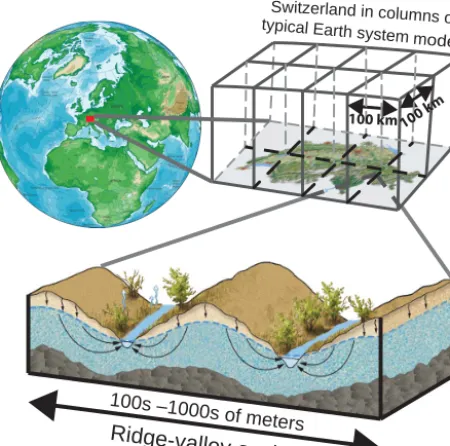
Figure 1.Sub-grid-scale surface heterogeneity and subsurface wa-ter redistribution are unrepresented in Earth system models. At the 100 km by 100 km grid cell scale, large mountain ranges (such as the Swiss Alps) become indistinct.

ual ridges and valleys disappear, and even major mountain ranges and basins can become indistinct. Likewise, much of the variability in the surface climatology of the landscape and its consequences for land–atmosphere interactions are lost.

This loss of detail in land surface properties has impor-tant implications for water fluxes in Earth system models. Given that ET may depend nonlinearly on both water avail-ability and atmospheric water demand, which are both spa-tially variable at scales far below typical model grid scales, the average ET over a heterogeneous landscape may differ substantially from model ET estimates derived from spatially averaged land surface properties. The potential importance of this issue has motivated research into methods for captur-ing sub-grid-scale properties and processes within Earth sys-tem models. For example, Beven (1995) discussed the scale dependence of hydrological models and the pitfalls of using effective parameters to reproduce the areal averages of sub-grid fluxes, especially where water availability strongly influ-ences the vapor flux. These aggregation problems arise from the nonlinearity of the governing processes, together with the spatial heterogeneity of the system.

Nesting higher-resolution regional models within global models represents an obvious, but computationally demand-ing, approach to treating sub-grid-scale heterogeneity. As de-scribed by Klink (1995), two broad classes of aggregation schemes have been proposed to incorporate sub-grid hetero-geneity while keeping computational costs manageable. In “averaged” surface schemes, the surface properties are aver-aged over each grid cell and the average is applied directly

in the model. In “mosaic” schemes, by contrast, individual grid cells are partitioned into several surface types, the model is run for each surface type separately, and the fluxes from each surface type are area weighted to determine the average fluxes for the grid cell.

Numerous modeling studies over the past two decades have shown that, in comparison to mosaic schemes and nested high-resolution models, averaged surface schemes tend to overestimate evapotranspiration and sensible heat flux (e.g., Klink, 1995; Giorgi and Avissar, 1997; Essery et al., 2003; Teluguntala et al., 2011; Ershadi et al., 2013). Stud-ies with nested high-resolution models demonstrate that this overestimation bias is largest where topographic effects play a major role (Giorgi and Avissar, 1997; Pope and Stratton, 2002; Boyle and Klein, 2010; Bacmeister et al., 2014).

Another potential source of bias in Earth system mod-els arises from their neglect of surface and subsurface flows within and between grid cells. Current Earth system mod-els calculate infiltration and vertical transport of water in each soil column, but the water that reaches the bottom of the column is either stored as groundwater or simply dis-appears, reappearing later in the ocean. In real-world land-scapes, by contrast, significant volumes of water are trans-ported laterally, either via groundwater flow or by rivers flow-ing from mountains into valleys and potentially redistribut-ing their water to valley ecosystems by infiltration into valley aquifers. These lateral redistribution processes supply water for evapotranspiration in groundwater-dependent ecosystems in the dry season (Fan and Miguez-Macho, 2010). Several case studies in the Amazon (Christoffersen et al., 2014), cen-tral Argentina (Contreras et al., 2011; Jobbágy et al., 2011), and other groundwater-dependent ecosystems (Eamus et al., 2015) demonstrate how water supply can govern the season-ality and magnitude of evapotranspiration in those regions. However, the potential effects of these lateral redistribution processes on grid-scale ET, as viewed from the atmosphere, are missing from current Earth system models, and the re-sulting biases in modeled water fluxes are unknown.

estimates of the potential effects of sub-grid heterogeneity and subsurface lateral redistribution on ET fluxes from het-erogeneous landscapes, as seen from the atmosphere.

2 A Budyko framework for estimating terrestrial water partitioning

The simplest widely used approach for estimating evapotran-spiration rates from the land surface is the Budyko frame-work (Turc, 1954; Mezentsev, 1955; Pike, 1964; Budyko, 1974; Fu, 1981; Milly, 1993; Zhang et al., 2001; Yang et al., 2007). Budyko showed empirically that under steady-state conditions in catchments without significant groundwater in-puts, losses, or storage changes, the long-term annual av-erage evapotranspiration (ET) rate is functionally related to both the supply of moisture from the atmosphere (precipita-tion,P) and net irradiance (available energy) as an estimator of the evaporative demand for water by the atmosphere (po-tential evapotranspiration, PET). Under arid conditions (that is, whenP is much smaller than PET), ET converges toward

P, implying that ET is limited by the available supply of water (Fig. 2, water limit line). Alternatively, under humid conditions (that is, whenP is much greater than PET), ET is limited by atmospheric demand andEconverges toward PET (Fig. 2, energy limit line). Budyko’s original work showed, and decades of studies have confirmed, that, under the long-term steady-state assumptions outlined above, hydrological systems typically operate close to either the energy or water constraints.

Several studies have explored how natural systems may violate the assumptions of the Budyko approach. Net inputs or losses of groundwater, as well as long-term changes in soil moisture and groundwater storage, have been shown to alter the water balance sufficiently that measurements of P and ET can produce points that fall far from the energy and water constraints in Fig. 2. However, these apparent violations of the Budyko approach can be corrected if the precipitation termP is replaced by an effective precipitation that accounts for root zone water storage changes and net inputs or losses of groundwater (Zhang et al., 2001, 2008; O’Grady et al., 2011; Istanbulluoglu et al., 2012; Wang, 2012; Chen et al., 2013; Troch et al., 2013; Du et al., 2016).

The Budyko framework can be expressed in two differ-ent non-dimensional sets of axes, depending on whether one wishes to focus on the effects of changing water supply (P) or atmospheric water demand (PET). If one seeks to analyze the effects of changing PET under a fixedP, it is most in-tuitive to non-dimensionalize both axes by P, as shown in Fig. 2a. In this coordinate space, translation along the hori-zontal axis represents a change in PET.

Our analysis, by contrast, focuses on how changes in wa-ter availability affect ET under a fixed PET. For such ques-tions, it is most intuitive to non-dimensionalize the coordi-nate axes by PET, as shown in Fig. 2b. In this coordicoordi-nate

space, translation left or right along the horizontal axis rep-resents changes in water availability. Thus, this coordinate space is better suited to our analysis.

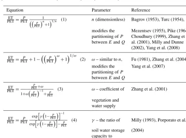
Table 1 presents several alternative empirical equations that have been proposed for “Budyko curves” relating ET to P and PET. Our analysis will be based on the Turc– Mezentsev equation (Eq. 1 in Table 1), because it is the most widely used of the alternatives shown here. However, the dif-ferences among these formulas are unimportant for the anal-ysis presented below.

Here, we use Budyko curves as simple models for how ET is controlled by the supply of available moisture (as rep-resented byP) and evaporative demand (as represented by PET). We could have used more complex ecohydrological models to estimate ET instead, at the cost of increased com-plexity and reduced transparency. However, any such mod-els must obey the same energy and water constraints that shape the behavior of catchments in the Budyko framework, so we would not expect their behavior to deviate greatly from the Budyko curves that are analyzed here. Thus, the Budyko curves that we analyze here can be considered as approxima-tions to the behavior of these more complex models. They also have an important advantage for our purposes, namely that they specify ET as an explicit function of its main drivers

P and PET, allowing us to derive general analytical results that might otherwise be difficult to infer from sets of simula-tion results.

3 Effects of sub-grid heterogeneity on ET in a Budyko framework

The water and energy constraints that limit ET imply that ET is an intrinsically nonlinear function ofP and PET. Un-der arid conditions (withPPET), ET will increase almost linearly withP, but as conditions become more humid and the supply of moisture exceeds the energy available to evap-orate it (PPET), the energy constraint will hold ET nearly constant asPincreases. Conversely, under humid conditions, ET will scale almost linearly with evaporative demand (as ex-pressed by PET), but as conditions become more arid and the supply of moisture becomes limiting, ET will be constrained byP and will become largely independent of PET.

As shown in Fig. 3, the nonlinear behavior of ET as a func-tion ofP and PET is also reflected in Budyko curves, partic-ularly near the transition between humid and arid conditions (P/PET close to 1). This nonlinear behavior has important implications for estimates of average ET in heterogeneous landscapes.

Figure 2.Budyko framework and energy and water limit lines. The blue cloud is a smoothed scatterplot of the 30 arcsec resolution mean annual precipitation (P), evapotranspiration (ET), and potential evapotranspiration (PET) for continental Europe. ET and PET data are from MODIS (Mu et al., 2007),P data set is from WorldClim (Hijmans et al., 2005).

Table 1.Alternative empirical equations for mean annual evaporation rate in Budyko framework: ET is mean annual evapotranspiration,Pis mean annual precipitation, PET is mean annual potential evapotranspiration (evaporative demand).

Equation Parameter Reference

ET PET=

P

PET 1

P PET

n +1

1/n (1) n(dimensionless) Bagrov (1953), Turc (1954),

modifies the Mezentsev (1955), Pike (1964) partitioning ofP Choudhury (1999), Zhang et betweenEandQ al. (2001), Milly and Dunne

(2002), Yang et al. (2008)

ET

PET=PETP +1−

P

PET

ω +1

1/ω

(2) ω– similar ton, Fu (1981), Zhang et al. (2004), modifies the Yang et al. (2007)

partitioning ofP

betweenEandQ

ET PET=

P PET+ω 1+ω

P PET

−1 +_PETP

(3) ω– coefficient of Zhang et al. (2001)

vegetation and water supply

ET PET=PETP

exp

h γ

1−_PETP

i−1

exphγ1− P PET

i

− P PET

(4) γ– the ratio of Milly (1993), Porporato et al.

soil water storage (2004) capacity to

precipitation

the resulting heterogeneity bias will depend on how strongly curved the function is, and how widely its inputs are scat-tered. This intuitive concept can be expressed mathemati-cally by comparing the value of the function, and the mean of its second-order Taylor expansion around the same point, to estimate the heterogeneity bias (e.g., Kirchner et al., 1993).

We begin by restating Eq. (1) from Table 1 as an explicit function ofP and PET:

ET=f (P ,PET)= P

P

PET n

+1

1/n. (5)

approxi-ET

=

f

(P

, PET)

P/ PET

True average

of ET values

Average ET predicted

from average P/ PET

Heterogeneity

bias

loc. 2

loc.1

Figure 3. Illustration of heterogeneity bias in a Budyko curve (Eq. 5). The true average (gray circle) of the ET values of loca-tions 1 and 2 (black dots) is less than the average ET that would be estimated from their averageP/PET (open circle). The size of the heterogeneity bias will be proportional to the curvature in the ET function and proportional to the variability inP and PET among the individual points (Eqs. 6–8).

mation for the mean of the function, in terms of the function’s value at the mean of its inputs:

ET≈f P ,PET

+1

2

∂2f

∂P2var(P )+ 1 2

∂2f

∂PET2var(PET)

+ ∂

2_f

∂P ∂PETcov(P ,PET), (6)

where the derivatives are understood to be evaluated at P

andP ET. Evaluating the necessary derivatives using Eq. (5) directly yields the following expression for the average ET:

ET≈f P ,PET−(n+1) P n+1

PETn+1

Pn+PETn2 +1/n

×

₁ 2

var(P ) P2

+1

2

var(PET)

PET2

−cov(P ,PET)

PPET

, (7)

where the second term represents the heterogeneity bias (that is, the difference between the average of the function and the function of the average). The relative magnitude of this bias can be derived by combining Eqs. (7) and (5), yielding

f P ,PET₋ ET

f (P ,PET)

≈ (n+1)

P

PET n₂

+PET P

n₂2

×

₁ 2

var(P ) P2

+1

2

var(PET)

PET2

−cov(P ,PET)

PPET

. (8)

From Eq. (8) one can directly see that the heterogeneity bias will depend on the variances ofP and PET, as well as their covariance (all non-dimensionalized by their means). One can see that the heterogeneity bias will generally be positive (that is, estimates based onP and PET will overestimate ET), because the covariance term in Eq. (8) will be less than the variance terms. One can also see that, all else equal, a nega-tive correlation betweenP and PET will amplify the hetero-geneity bias (because, in terms of the Budyko plot, this will lead to greater scatter inP/PET). Furthermore, one can see that the relative heterogeneity bias will be greatest when the term in curly brackets in Eq. (8) will be as small as possi-ble, which will occur atP /PET=1 (the point of maximum curvature in the Budyko curve). Finally, from Eq. (8) one can see that at higher values ofn, the peak heterogeneity bias will be greater (due to then+1 term), but will be more tightly fo-cused aroundP /PET=1 (due to the powers ofn/2).

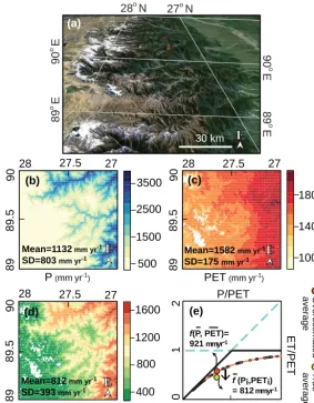
To estimate the heterogeneity bias that could result from grid-scale averaging in Earth system models, we applied the analysis outlined above to a 1◦by 1◦grid cell spanning the Himalayan Front in west Bhutan (Fig. 4a). This grid cell spans a sharp north–south topographic gradient, with alti-tudes ranging between∼500 and∼6500 m. Within this grid cell, we compiled 30 arcsec values of P (WorldClim; Hij-mans et al., 2005) and PET (MODIS; Mu et al., 2007) to ex-amine the finer-scale climatic drivers of variations in ET. Be-cause 30 arcsec is approximately 1 km, we will refer to these as 1 km values for simplicity.P and PET values at 1 km res-olution, as well as 1 km values of ET estimated from theseP

and PET data using the Budyko curve (Eq. 5), vary strongly in this 1◦by 1◦grid cell, as shown in Fig. 4b–d. The aver-ages of theseP, PET, and ET values over the 1◦_{by 1}◦_grid cell will plot as the yellow circle in Fig. 4e, lying well be-low the Budyko curve of the individual 1 km ET estimates. If instead we estimated the average ET for the grid cell from its averageP and PET, we would obtain the orange circle on the Budyko curve, corresponding to an 11.8 % overestimate of the true average of the 1 km ET values.

We repeated the same procedure to estimate the averag-ing bias in the eight grid cells surroundaverag-ing the one analyzed above (Fig. 5a). A comparison of these nine grid cells shows that the averaging error is largest (around 13 %) when the variability in the aridity index (AI=P/PET), driven in turn by topographic variability, is largest (Fig. 5b–d).

4 Lateral redistribution by surface and subsurface flow, and its effects on average ET in a Budyko framework

re-30 km

E

27o N 28o N

89

o

E

90

o

E

89

o E

90

o E

1600

1200

800

400 27

28 27.5

89

89.5

ET Budyko (mm yr-1₎

90

P/PET

ET/PET

01

2

0 1 2

f(P, PET)=

921mmyr-1

f (Pi,PETi)

= 812mmyr-1

Mean=812mm yr-1

SD=393mm yr-1

Overestimated

average

T

rue

average

E

(a)

27

28 27.5

89

89.5

PET (mm yr-1

)

90

1000 1400

Mean=1582mm yr-1

SD=175mm yr-1

1800

E

(c)

3500

2500

1500

500

P (mm yr-1

)

27

28 27.5

89

89.5

90

Mean=1132mm yr-1

SD=803mm yr-1

E

(b)

(d) (e)

Figure 4.One-kilometer topography (a: SRTM; Jarvis et al., 2008) and annual mean climatology for a 1◦by 1◦ grid cell spanning the Himalayan Front at 89–90◦E, 27–28◦N. Spatial patterns of 1 km resolution mean annual precipitation (b: WorldClim; Hijmans et al., 2005), potential evapotranspiration (c: MODIS; Mu et al., 2007), and(d)evapotranspiration (ET) calculated using the Budyko curve (Eq. 5). Panel

(e)shows a random sample of 50 points from(b),(c), and(d), along with the averageP, PET, and ET over the grid cell (yellow circle), and the ET value estimated from Eq. (5) for the same averageP and PET (orange circle). This ET estimate is 921 mm yr−1, 11.8 % more than the average of the 1 km resolution ET estimates.

PET₁ ET₁

P

P

2 ET₂

R

R

Drainage to

deep GW or

streamflow

Col. 1

Col. 2

Lateral transfer

0

0.5

1

0

1

2

3

4

Energy limit

Water limit

Col.2

Col.1

Available water/PET

ET/PET

Avg. without transfer

(a)

(b)

Avg. with transfer

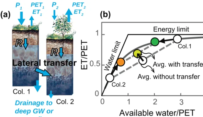
Figure 6. (a)A conceptual two-column model.(b)Illustration of how the two points representing the two columns shift towards each other in Budyko space if water is transferred from the upper, wetter column to the lower, drier column. Open circles represent columns without lateral transfer and solid circles represent columns with lateral transfer.

infiltrates into valley aquifers. The lateral transfer of water from the mountains to the valley could clearly increase evap-otranspiration rates in the valley by making more water avail-able for vegetation, but could simultaneously make less water available for transpiration in the mountains. Will the net ef-fect of this lateral transfer be to increase, or decrease, average ET as seen from the atmosphere?

The mountains, the valley, and the lateral transfer between them will all be invisible at the grid scale of typical Earth system models. But the simple scenario described above sug-gests that lateral transport could alter the average ET over a model grid cell that incorporated both the mountains and the valley. What properties of the landscape will control the sign and the magnitude of the net effect on average ET? Here, we extend the Budyko analysis presented above to estimate the potential effects of lateral redistribution on average ET as seen from the atmosphere.

Our first step is to redefine the aridity index in the Budyko framework to take account of water that becomes available for evapotranspiration either through local precipitation or through net lateral transfer. In taking this step, we are im-plicitly assuming that all water supplied to the ecosystem, from any source, is equally available for evapotranspiration. We introduce the term available water (AW), defined as

AW=P+net transfer, (9)

where net transfer represents the net influx of groundter and re-infiltrating streamflow. Substituting available wa-ter for precipitation in the Turc–Mezentsev formula for the Budyko curve (Eq. 5), we obtain

ET= AW

AW PET

n

+1 1/n =

P+net transfer

P+net transfer PET

n

+1

1/n, (10)

where AW is available water and, as before, ET is actual evapotranspiration,P is precipitation, PET is potential evap-oration, andn(dimensionless) is a catchment-specific param-eter that modifies the partitioning ofP betweenE andQ. Our approach follows the lead of several other investigators (Istanbulluoglu et al., 2012; Wang, 2012; Chen et al., 2013; Du et al., 2016) who have expanded the “precipitation” term to account for other sources of water in addition to precipita-tion per se. This approach assumes that lateral transfer alters only the available water at the two locations, and not their PETs.

will the average ET as seen from the atmosphere increase or decrease, and by how much?

We can graphically illustrate the effects of lateral redistri-bution between the two columns in the Budyko framework as shown in Fig. 6b. The average ET of Column 1 and Col-umn 2 will always lie on the line connecting the correspond-ing points on the Budyko plot (and thus below the Budyko curve itself). As Fig. 6b shows, if we laterally transfer wa-ter from a more humid column to a more arid column, the corresponding points on the Budyko plot must move closer together, and the resulting average ET must move upward. Conversely, if we laterally transfer water from a more arid column to a more humid one, the corresponding points on the Budyko plot must move farther apart, and the average ET must decrease.

Because lateral transfer will necessarily be driven by grav-ity (and thus source locations will always lie above recipient locations), the analysis shown in Fig. 6b leads directly to a simple general rule: wherever higher locations are more hu-mid, one should expect lateral redistribution to result in a net increase in ET, and conversely, wherever higher locations are more arid, lateral redistribution should result in a net de-crease in ET.

As one can see from the graphical analysis shown in Figs. 6 and 7, the magnitude of the net ET effect will depend primarily on the amount of lateral redistribution (how far the points move along the Budyko curve) and on the degree of curvature between them (and thus the angle between the tra-jectories of the individual points). As shown in Fig. 7, if both locations are humid (and thus energy limited) or both loca-tions are arid (and thus water limited), lateral transfer from one site to the other will have only a minimal effect on the average ET. If both sites are energy limited (and remain en-ergy limited), neither will respond strongly to a change in the amount of water available for evapotranspiration. If both sites are water limited (and remain water limited), they will be al-most equally sensitive to changes in available water; thus, the increases in available water and ET at one site will be nearly offset by the corresponding reductions at the other site. But if one site is water limited and the other is energy limited, then the responses of the two sites to changes in available water will be markedly different, and lateral transfer from one to the other could substantially affect the average ET over the two sites.

We emphasize that the analysis presented here is hypothet-ical. We are not asserting that lateral transfer actually occurs between the two columns, or even that it can occur between them, let alone what the magnitude of that lateral transfer is. Instead, we are asking the hypothetical question: if water flows from one column to the other, how much would we ex-pect the average ET to change, for each mm yr−1 of water that is lost from one column and gained by the other?

> 0

0.5

0 1 2 3 4

Energylimit Available water/PET ET/PET 1 Col.1 Col.2 Water limit AW1 PET1 AW2 PET2 (a) 0 0.5 1

0 1 2 3 4

Energylimit

Water limit

< Col.1

Col.2

ET/PET AW1 PET1 AW2 PET2 Available water/PET (b) Col.2 Col.1 ET/PET Available water/PET Water limit

0 1 2 3

(c) 4 Energy limit 0 0.5 1 ET/PET Available water/PET Water limit

0 1 2 3

(d) 4 Energy limit 0 0.5 1 Col.1 Col.2 Subsurface lateral flow ET1P1 _P

2

ET2

Column1Column2

Figure 7.Four conceptual cases in a two-column model where Col-umn 1 is topographically always higher than ColCol-umn 2 (water al-ways moves from Column 1 to Column 2). Open circles represent columns without lateral transfer and solid circles represent columns with lateral transfer. Depending on the columns’ wetness or dry-ness (P and PET), lateral transfer can potentially(a)increase av-erage ET (the points representing Column 1 and Column 2 are pushed towards one another, spanning significant curvature in the ET function),(b) decrease average ET (points are pushed away from one another, spanning significant curvature in the ET func-tion), or(c, d)have little effect on average ET (the columns shift almost collinearly along the energy-limit or water-limit limbs of the curve).

4.2 Quantifying the effect of lateral transfer on average ET

We can make a first-order estimate of the net effect on ET using the Budyko curve as a simple model of ET rates. An illustrative calculation, for an extreme hypothetical case, is shown in Fig. 8. Column 1 is humid, with 2000 mm yr−1of annual precipitation and a PET of 1000 mm yr−1_{(AI of 2.0),} and Column 2 is arid, with 300 mm yr−1 _{of annual} precipi-tation and a PET of 2000 mm yr−1(AI of 0.15). As Fig. 8b shows, laterally transferring 200 mm yr−1from Column 1 to Column 2 would increase average ET by about 85 mm yr−1, or 14 %.

We can generalize from this specific example by using Eq. (10) to calculate the average ET as a function of the amount of available water that is transferred from one col-umn to the other:

ETavg=0.5 



(P1−x)×PET1

(P1−x)n+PETn1

1_n

+ (P2+x)×PET2

(P2+x)n+PETn2

_n1 

,

in-Valley

P1= 2000

mm yr-1

P2= 300

mm yr-1

PET1=1000 mm yr-1

ET2= 297

mm yr-1

ET1=894

mm yr-1 PET2=2000 mm yr-1 ETavg= 595 mm yr-1

(a) Without lateral transfer

Column 2 Column 1

R1=1106mm yr-1 R2=3 mm yr -1

D

D

Mountain

P1= 2000

mm yr-1

PET1=1000 mm yr-1

ET’_{mm yr}1=874_-1

P2= 300

mm yr-1 ET’2= 485

mm yr-1 PET2=2000 mm yr-1 ET’avg= 680 mm yr-1~14 %

(b) With lateral transfer

D

D

Transfer=200

mm yr-1

Column 1

Column 2

R’1=926mm yr-1 _R’

2=15mm yr-1

~

Mountain

_Valley

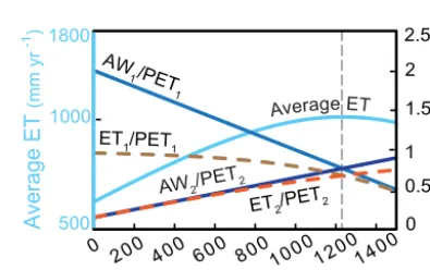
Figure 8.Hypothetical numerical experiment with conceptual two-column model:(a)no lateral transfer between columns,(b)200 mm yr−1 lateral transfer from Column 1 (mountain) to Column 2 (valley) increases average ET by 14 %. The magnitude ofP (precipitation), PET (potential evapotranspiration), ET (actual evapotranspiration), andR(recharge) are hypothetical andDis drainage to deep groundwater or streamflow.

creasing net transfer (x) up to a point, and then decreases for higher values ofx. One can see from Fig. 9 that average ET reaches its maximum whenx equalizes AW / PET (and thus ET / PET) at the two sites (note that this does not imply that either AW or PET are necessarily the same at the two sites).

We can verify this intuitive result by differentiating Eq. (11) byx:

dETavg dx =

1

P2+x PET2

n

+1 1+1/n−

1

P1−x PET1

n

+1 1+1/n.

(12) At the maximum ETavg, dETavg/dx must equal zero, which can only occur if xopt, the ET-maximizing rate of lateral transfer, is such that the two terms in Eq. (12) are equal, im-plying that

_P 1−xopt PET1

n

+1=

_P 2+xopt

PET2 n

+1→

P1−xopt PET1

=P2+xopt

PET2

= P1+P2

PET1+PET2

, (13)

which shows directly that AW/PET=(P±xopt)/PET in the two columns must be equal, confirming the intuitive result from Fig. 9. Solving Eq. (13) forxoptleads to

xopt=

P1PET2−P2PET1 PET1+PET2

=P1/PET1−P2/PET2

1/PET1+1/PET2

. (14)

The key result here (namely that ET is maximized when lat-eral transfer equalizes the ratio AW / PET in the columns) is not restricted to two columns, and is not specific to the par-ticular curve that we have analyzed here. Instead, it can be

0 0.5 1.5 2 2.5 500 1000 1800

200 400 600 800100012001400 Net transfer (mm yr-1₎

Av er ag e ET (mm yr -1 ) AW 1/PET 1

ET1/PET1 ₁

0

ET/PET

, A

W/PET

ET2/PET2

AW2/PET2

Average ET

Figure 9.Average ET is maximized for the rate of net transfer at whichP/PET and ET/PET of the two hypothetical columns of Fig. 8 cross one another.

shown to be true for any downward-curving function on a Budyko plot and for any number of interacting columns; for details, see the Appendix.

The dimensionless quantity dETavg/dx (Eq. 12) expresses the change in average ET per unit of lateral redistribu-tion. One quantity of particular interest could be the relative change in ET resulting from the first unit of lateral transfer, which can be obtained directly from Eq. (12) withx=0:

dETavg dx

atx=0

= 1 P2 PET2 n +1 1+1/n

− 1 P1 PET1 n +1

This dimensionless number depends only on the aridity in-dicesP/PET at the two sites, and could be used as a screen-ing tool to find regions where lateral redistribution could po-tentially be most consequential.

Another benchmark for the potential importance of lateral transfer is the maximum possible average ET rate, if lateral transfer took place at its optimal valuexopt. This quantity can be calculated by substituting the optimal transfer rate xopt (Eq. 14) into our modified Budyko formula (Eq. 11):

ETopt=

P1+P2 2

P1+P2 PET1+PET2

n

+1

1/n. (16)

Equation (16) shows that the optimal rate of ET (including lateral redistribution) equals the Budyko curve estimate of ET at the averageP and average PET. As shown in the Ap-pendix, this result is quite general, and does not depend on the specific Budyko curve equation that we have used here, nor on any specific number of columns. It requires only that all of the columns are governed by the same downward-curving function in a coordinate space defined by ET/PET andP/PET.

This result demonstrates an interesting connection with the analysis of heterogeneity bias presented above. The maxi-mum possible increase in ET from lateral redistribution ex-actly equals the heterogeneity bias calculated in the preced-ing section: both are equal to the ET function at the average

P and PET (e.g., Eq. 16 in the case of two columns), minus the average of the ETs calculated for the individual columns using their individual P and PET values. That is, both are equal to “the function of the averages”, minus “the average of the functions”. Putting the same point differently, the ET that an Earth system model calculates from averageP and PET (the function of the averages) is not just an overestimate of the true ET (as explained in Sect. 3 above); it is the high-est possible ET under optimal redistribution of the available water.

This observation simplifies the problem of estimating the maximum possible effect of lateral redistribution in hetero-geneous terrain: one simply needs to compare the average of the ETs calculated for every pixel within some domain using those pixels’ individual P and PET values, and the ET calculated from the average P and average PET using the same Budyko curve. Alternatively, one can approximate these quantities from the means and variances ofP and PET, using Eqs. (6)–(8).

Of course, any of these estimates of the potential effects of lateral redistribution ignore many real-world constraints, such as topographic or lithologic barriers that could prevent lateral transfer between specific locations (e.g., water will not flow uphill). Thus, this estimate should be considered as only a theoretical upper bound.

4.3 Real-world example of redistribution effects on estimated ET

To illustrate the possible effects of lateral redistribution on average ET in the real world, we will use the example of the 1◦by 1◦grid cell shown in the middle right of Figs. 4a and 5a, which lies at the foot of the Himalayan Front at 89– 90◦E, 26–27◦N. As before, we use 30 arcsec (∼1 km) P, PET, and topographic data (from WorldClim, MODIS, and SRTM; Hijmans et al., 2005; Mu et al., 2007; Jarvis et al., 2008) to represent the finer-scale heterogeneity within this grid cell.

Figure 10 shows three locations that have been selected to illustrate the possible effects of lateral redistribution on average ET. Location 3 is close to sea level, whereas loca-tion 2 is at 300 m altitude and localoca-tion 1 is at roughly 3000 m. We analyzed the effects of a hypothetical redistribution of 500 mm yr−1of water from location 1 to location 2, and from location 2 to location 3.

As Fig. 11 shows,P and the aridity index increase dramat-ically from location 1 (at 3000 m) to location 2 (at 300 m); that is, the landscape becomes more humid as one moves downhill. Using the rule of thumb developed above, one would expect that lateral transfer from location 1 to loca-tion 2 should result in a net decrease in average ET. Fig-ure 12a confirms that, as expected, lateral transfer would move the two points farther apart on the Budyko curve, re-sulting in a net decrease of 9.3 % in the average ET of the two locations.

Conversely, as Fig. 11 shows, as one moves downhill from location 2 to location 3, the landscape becomes more arid (the aridity index decreases); thus, the rule of thumb outlined above predicts that downhill lateral transfer should result in a net increase in average ET. This expectation is confirmed by Fig. 12b; the two locations move closer together on the Budyko curve, resulting in a net 4 % increase in the average ET of the two locations.

5 Summary and discussion

The atmosphere mixes and integrates inputs from spatially heterogeneous landscapes. Earth system models average over significant landscape heterogeneity, which can lead to sub-stantial biases in model results if the underlying equations are nonlinear. Due to the mass and energy constraints that limit evapotranspiration rates, ET will be a nonlinear concave-downward function of P and PET, whether expressed by Budyko curves or by other ET models. As a result, ET val-ues calculated from averages of spatially varyingP and PET will overestimate the average of the spatially variable ET (the function of the average will overestimate the average of the function).

26

27 26.5

89

89.5

90

100300 500 1000 2000 3000

26

27 26.5

89

89.5

90

0.5 1.0 1.5 2.0 2.5

Altitude

Aridity index

26

27 26.5

89

89.5

90

Precipitation

26

27 26.5

89

89.5

90

Potential ET

1000 2000 3000 4000

1800 2000 2200 2400 2600

PCP (m yr1 2 3 4 5-1₎ Altitude (km)

0 1 2 3

PET (m yr-1₎

1.8 2.2 2.6 Aridity 0.5 1.5 2.5

1 2

3

(a)

(b)

(c)

(d)

Figure 10.Spatial patterns of altitude, precipitation (P), potential evapotranspiration (PET), and aridity index (P/PET) in 1◦by 1◦grid cell in the Himalayas at 89–90◦E, 26–27◦N. There is a sharp gradient inP, PET, and altitude in this grid cell. The labeled points 1, 2, and 3 correspond to the labeled points in Fig. 11.

Aridity index í

Altitude

NP

0.5 1.5 2.5

P (m yr-1

01

2

3

Altitude

NP

Altitude

NP

PET (m yr-1

1.8 2.2 2.6

1 2 3 4

01

2

3

0

12

3

1.8 2.2 2.6

PET (m yr-1

P

(m yr

-1

12

3

4

3 2

1

300 m ₂

1

3 3 2

1

3 2

1

(a) (b) (c) (d)

Figure 11.Variation of precipitation (P), potential evapotranspiration (PET), and aridity index (P/PET) with altitude in a 1◦by 1◦grid cell of the Himalayas in the extent of Fig. 4 (89–90◦E, 26–27◦N).P and PET for sites 1, 2, and 3 in Fig. 10 are marked in the graphs. Between locations 3 and 2,Pand aridity index increase and PET decreases with altitude. Between points 2 and 1,Pand aridity index sharply decrease and PET slightly increases with altitude.

empirical ET model. One should keep in mind that Budyko curves are empirically calibrated to catchment-averaged pre-cipitation and discharge (to calculate ET); thus, they al-ready average over the spatial heterogeneity within each cal-ibration catchment. This inherent spatial averaging should make Budyko curves smoother (less curved) than the point-scale relationships that determine ET as a function of P

and PET. In other words, the true mechanistic equations that drive point-scale ET may be much more sharply curved than Budyko curves (which already include significant averaging, and thus must plot inside the curve of the raw point-scale data, if such data were available). As a result, the effects of sub-grid heterogeneity and lateral redistribution could poten-tially be larger than what we have estimated here.

re-P/PET

ET/PET Energy limit

Wa

ter lim

it

01

2

0 1 2

Avg. ET

= - 9.3 % Avg. ET after transfer Avg. ET before transfer

2

1

2

1

(a)

P/PET

Energy limit

Wat

er li

mit

0 1 2

Avg. ET

= +4 % Avg. ET after transfer Avg. ET before transfer

2

3

2 3

(b)

Figure 12.Budyko curve and increase or decrease of average ET when transfer of water from a higher location to a lower location is included.(a)500 mm yr−1of transfer from site 1 (3000 m altitude, lower aridity index) to site 2 (300 m altitude, higher aridity index) decreases the average ET by 9.3 %. (b) 500 mm yr−1of transfer of water from location 2 (altitude 300 m, higher aridity index) to location 3 (altitude 10 m, lower aridity index) increases the average ET by 4 %.

gions where the aridity index decreases with altitude, lateral transfer would redistribute water from more arid uplands to more humid lowlands, resulting in a net decrease in average ET (Fig. 12a). We derived simple analytical formulas for es-timating the marginal ET effect of a unit of lateral redistri-bution, as well as the maximum possible ET effect resulting from an optimal (i.e., ET-maximizing) amount of lateral re-distribution. Water transfers will most strongly affect average ET if the source (or recipient) location is energy limited and the recipient (or source) location is water limited.

Our analysis of redistribution effects is based on the as-sumption that lateral transfers will reduce the available water at the source location by the same amount that they increase it at the receiving location. Thus, we are assuming that water that is redistributed becomes unavailable for evapotranspira-tion at the source locaevapotranspira-tion (for example, through rapid runoff to channels or rapid infiltration to deep groundwater via pref-erential flowpaths). Alternatively, if the redistributed water were assumed to come only from surplus that is left over af-ter evapotranspiration, the available waaf-ter (and thus ET) in the source location would not be reduced while the avail-able water (and thus ET) in the receiving location would be increased. Under that assumption, any redistribution would increase average ET, regardless of the climatic conditions in the source and receiving locations. By assuming that avail-able water is conserved (in the sense that whatever is gained in one location is lost from another), our analysis may under-estimate the effect of redistribution on average ET.

It bears emphasis that our analysis of the effect of lat-eral redistribution is inherently hypothetical. By estimating the ET effect of a (hypothetical) transfer of water from one location to another, we are not implying that such a trans-fer would actually take place at the assumed rate (or would

even occur at all) in the real world. Perhaps in reality there is no flowpath connecting the two locations, for example, or perhaps its conductivity is very low, or perhaps the putative source location lies downhill from the putative recipient loca-tion. Likewise, although there may be an aquifer connecting two locations, it may lie too deep below the rooting zone to have any significant impact on evapotranspiration rates. Esti-mating the potential effects of lateral redistribution on ET in real-world cases (rather than hypothetical ones) will require careful attention to such matters, which are beyond the scope of this paper.

The analysis that we have used to quantify the effects of spatial heterogeneity and redistribution could also be used to study the effects of temporal heterogeneity in water avail-ability for evapotranspiration, and temporal redistribution by storage of groundwater between wet and dry seasons. Temporal heterogeneity (e.g., seasonality) in water avail-ability could substantially affect average ET, particularly in climates that shift seasonally between water-limited and energy-limited conditions. In such cases, ET estimates cal-culated from time-averagedP and PET will be higher than the average of individual ET estimates derived from daily or monthly values for available water and PET. Similarly, temporal redistribution of available water between water-limited and energy-water-limited conditions (through, e.g., inter-seasonal groundwater storage) could substantially increase average ET. The formulas and approaches we have outlined above could be straightforwardly applied to quantify these temporal heterogeneity and redistribution effects (for a sim-ilar approach to temporal upscaling in hydrological models, see Lim and Roderick, 2014). If, however, one bases such an analysis on Budyko curves as an ET model, one should keep in mind that these empirical curves are based on long-term catchment mass balances, and thus they already aver-age over seasonal and shorter-term variations in water avail-ability and PET. Thus, Budyko curves may already be sub-stantially smoother (less curved) than the short-term behavior that they average over. As a result, any such analysis based on Budyko curves may underestimate the impact of temporal heterogeneity and redistribution on average ET.

Our analysis does not explicitly account for how changes in ET may affect atmospheric humidity and thus PET. This “complementarity” feedback between ET and PET is poten-tially important for mechanistic models of the evapotranspi-ration process, and could potentially change the magnitude (though not the sign) of the ET effects that we have estimated in this paper. Any such changes should be small, however, because Budyko curves are empirical relationships derived from catchment mass balances, which already subsume any feedbacks between ET and PET that arise in the calibration catchments.

more complex ecohydrological models. On the other hand, it avoids the calibration issues and data constraints that may limit the applicability of these more complex models. Our simple approach also has the advantage of transparency; as Figs. 3, 4e, 6, and 12 show, one can directly visualize how both spatial heterogeneity and lateral redistribution affect av-erage ET, using a simple graphical framework. This frame-work leads to relatively simple analytical expressions and rules of thumb that can be used to gauge where, and when, heterogeneity and lateral redistribution effects on ET are likely to be most important.

An obvious next step is to use the framework developed here to make a first-order estimate of the likely effects of spatial heterogeneity and lateral redistribution on ET, as seen from the atmosphere at regional and continental scales. The approach developed here is well suited to this task because it is simple and relatively general, and its data requirements are modest. Heterogeneity effects on ET can be estimated from the means, variances, and covariance ofP and PET, and, as we have shown, the maximum hypothetical effect of lateral redistribution can be obtained directly from the same analy-sis. Quantifying the likely real-world effects of lateral redis-tribution will be much more challenging, since it necessarily requires estimating the real-world magnitudes of these lateral redistribution fluxes. Work on quantifying heterogeneity and redistribution effects on ET at regional and continental scales is currently underway and will be the focus of future papers.

6 Data availability

Appendix A: Generality of redistribution results Here, we demonstrate that the optimal redistribution results presented in Sect. 4.2 are also valid for any number of loca-tions (not just two) and for any downward-curving ET func-tion that can be plotted on the Budyko axes (not just Eq. 1, which was used to derive Eqs. 12–16 in Sect. 4.2).

We begin by assuming a set of N locationsi=1 . . . N, each characterized by rates of precipitation Pi and

poten-tial evapotranspiration PETi. In keeping with the analysis of

Sect. 4, we assume that the rate of evapotranspiration at each location depends on its available water, AWi:

available wateri=AWi =Pi±net transfers, (A1)

and specifically on the ratio of available water to PET, which we denote for future convenience asRi,

Ri=

AWi

PETi

. (A2)

We also assume that the evapotranspiration rates at all loca-tions follow the same functional dependence on AWi/PETi,

and that this functional relationship (denotedf) can be rep-resented on Budyko-type axes, that is,

ETi PETi =f _AW i PETi

=f (Ri)or ETi=PETif (Ri) . (A3)

We impose no restrictions on the form of the functionf, ex-cept that it must be downward-curving; that is, its second derivative must be negative everywhere.

The first result to be demonstrated is if moisture is redis-tributed among multiple locations, the highest possible aver-age rate of ET will be achieved when all locations have the same ratioRi=AWi/ PETi (note that this does not require

that the AWi or the PETi are the same). We begin by

as-signing all the locations the sameRvalue, which we denote

Ropt(recognizing that its optimality is not yet proven). We then show that any further redistribution of an amount of wa-tery from any locationj to any other locationk(such that

Rj< RoptandRk> Ropt) will necessarily lead to a decrease in overall ET. The transfer ofyfrom locationj to locationk

implies that

Rj=Ropt−

y

PETj , dRj

dy = −

1 PETj

(A4)

and

Rk=Ropt+

y

PETk , dRk

dy =

1 PETk

. (A5)

Taking the second-order Taylor expansion of Eq. (A3), one obtains for ETj

ETj=PETjf Ropt

+PETj df

dR

dR

dyy+

PETj 2

d2_f dR2

_d R

dy 2

y2+. . .

=PETjf Ropt+PETj df

dR

−1 PETj

y+PETj 2

d2_f dR2

₋

1 PETj

2

y2+. . .

=PETjf Ropt

−ydf

dR+ y2 2PETj

d2_f

dR2+. . ., (A6)

and similarly for ETk

ETk=PETkf Ropt+y df

dR+ y2

2PETk

d2f

dR2+. . .. (A7) Thus, the net change in total ET for locationsjandktogether is

ETj+ETk

−PETjf Ropt

+PETkf Ropt

=y2

₁

2PETj

+ 1

2PETk

_d2_f

dR2+. . .. (A8) Because the second derivative off is always negative, the right-hand side of Eq. (A8) will likewise be negative, imply-ing a net decrease in ET for locationsj andkwheneveryis not zero. The stipulation that the second derivative off is negative everywhere guarantees that any higher-order terms that have been omitted from the Taylor expansion must be too small to change the sign of the right-hand side of Eq. (A8).

Thus, the general result is demonstrated for the individ-ual pair of locationsj andk. Demonstrating that this result is true for this pair of locations is sufficient to prove the gen-eral case, since any pattern of water redistribution among any combination of locations is equivalent to a linear combina-tion of such pairwise water transfers.

The second result to be demonstrated is that, for any Budyko-type functionf and any combination of locations, the optimal rate of ET (including lateral redistribution among the locations) will equal the Budyko curve estimate at the av-erageP and average PET. For a set of locationsi, Eq. (A3) implies an average ET of

ET=PETif (Ri), (A9)

where overbars indicate averages over all locations. As demonstrated above, under optimal redistribution each loca-tion will haveRi=Ropt, such that Eq. (A9) becomes

ETopt=PETf Ropt. (A10)

What remains to be proven is thatRopt=P /PET. If we de-note the net transfer of water into each location aszi (such

that locations that have a net gain of available water have

zi>0, and locations that have a net loss of available water

havezi<0), for each location we can write Ri=

AWi

PETi

=Pi+zi

PETi

orRiETi=Pi+zi. (A11)

Summing Eq. (A11) over all locations, noting that under any mass-conserving redistribution thezivalues must sum to

zero and under optimal redistributionRi=Ropteverywhere, we directly obtain

X

RiPETi =Ropt X

PETi =

X

Pi+zi=

X

and therefore

Ropt= P

Pi

P PETi

= P

PET. (A13)

Combining Eqs. (A10) and (A13), we have

ETopt=PETf P

PET !

, (A14)

Author contributions. Both authors have contributed equally to all aspects of this work.

Competing interests. The authors declare that they have no conflict of interest.

Acknowledgements. We thank Ying Fan Reinfelder for insightful discussions, and Ross Woods, Michael Roderick, and two anony-mous reviewers for their comments.

Edited by: R. Woods

Reviewed by: M. Roderick and two anonymous referees

References

Bacmeister, J. T., Wehner, M. F., Neale, R. B., Gettelman, A., Han-nay, C., Lauritzen, P. H., Caron, J. M., and Truesdale, J. E.: Ex-ploratory High-Resolution Climate Simulations using the Com-munity Atmosphere Model (CAM), J. Climate, 27, 3073–3099, doi:10.1175/JCLI-D-13-00387.1, 2014.

Bagrov, N. A.: Mean long-term evaporation from land surface, Me-teorol. Gidrol., 10, 20–25, 1953.

Beven, K.: Linking parameters across scales: Subgrid parameteriza-tions and scale dependent hydrological models, Hydrol. Process., 9, 507–525, doi:10.1002/hyp.3360090504, 1995.

Boyle, J. and Klein, S. A.: Impact of horizontal resolution on cli-mate model forecasts of tropical precipitation and diabatic heat-ing for the TWP-ICE period, J. Geophys. Res.-Atmos., 115, D23113, doi:10.1029/2010JD014262, 2010.

Budyko, M. l.: Climate and life, Academic, New York, 1974. Chen, X., Alimohammadi, N., and Wang, D.: Modeling interannual

variability of seasonal evaporation and storage change based on the extended Budyko framework, Water Resour. Res., 49, 6067– 6078, doi:10.1002/wrcr.20493, 2013.

Choudhury, B. J.: Evaluation of an empirical equation for annual evaporation using field observations and results from a bio-physical model, J. Hydrol., 216, 99–110, doi:10.1016/S0022-1694(98)00293-5, 1999.

Christoffersen, B. O., Restrepo-Coupe, N., Arain, M. A., Baker, I. T., Cestaro, B. P., Ciais, P., Fisher, J. B., Galbraith, D., Guan, X., Gulden, L., van den Hurk, B., Ichii, K., Imbuzeiro, H., Jain, A., Levine, N., Miguez-Macho, G., Poulter, B., Roberti, D. R., Sakaguchi, K., Sahoo, A., Schaefer, K., Shi, M., Ver-beeck, H., Yang, Z.-L., Araújo, A. C., Kruijt, B., Manzi, A. O., da Rocha, H. R., von Randow, C., Muza, M. N., Borak, J., Costa, M. H., Gonçalves de Gonçalves, L. G., Zeng, X., and Saleska, S. R.: Mechanisms of water supply and vegetation de-mand govern the seasonality and magnitude of evapotranspira-tion in Amazonia and Cerrado, Agr. Forest Meteorol., 191, 33– 50, doi:10.1016/j.agrformet.2014.02.008, 2014.

Clark, M. P., Fan, Y., Lawrence, D. M., Adam, J. C., Bolster, D., Gochis, D. J., Hooper, R. P., Kumar, M., Leung, L. R., Mackay, D. S., Maxwell, R. M., Shen, C., Swenson, S. C., and Zeng, X.: Improving the representation of hydrologic processes in Earth System Models, Water Resour. Res., 51, 5929–5956, doi:10.1002/2015WR017096, 2015.

Contreras, S., Jobbágy, E. G., Villagra, P. E., Nosetto, M. D., and Puigdefábregas, J.: Remote sensing estimates of supplementary water consumption by arid ecosystems of central Argentina, J. Hydrol., 397, 10–22, doi:10.1016/j.jhydrol.2010.11.014, 2011. Du, C., Sun, F., Yu, J., Liu, X., and Chen, Y.: New

interpreta-tion of the role of water balance in an extended Budyko hy-pothesis in arid regions, Hydrol. Earth Syst. Sci., 20, 393–409, doi:10.5194/hess-20-393-2016, 2016.

Eamus, D., Zolfaghar, S., Villalobos-Vega, R., Cleverly, J., and Huete, A.: Groundwater-dependent ecosystems: recent insights from satellite and field-based studies, Hydrol. Earth Syst. Sci., 19, 4229–4256, doi:10.5194/hess-19-4229-2015, 2015. Ershadi, A., McCabe, M. F., Evans, J. P., and Walker, J. P.:

Effects of spatial aggregation on the multi-scale estimation of evapotranspiration, Remote Sens. Environ., 131, 51–62, doi:10.1016/j.rse.2012.12.007, 2013.

Essery, R. L. H., Best, M. J., Betts, R. A., Cox, P. M., and Taylor, C. M.: Explicit Representation of Subgrid Heterogeneity in a GCM Land Surface Scheme, J. Hydrometeorol., 4, 530–543, doi:10.1175/1525-7541(2003)004<0530:EROSHI>2.0.CO;2, 2003.

Fan, Y. and Miguez-Macho, G.: Potential groundwater contribu-tion to Amazon evapotranspiracontribu-tion, Hydrol. Earth Syst. Sci., 14, 2039–2056, doi:10.5194/hess-14-2039-2010, 2010.

Fu, B. P.: On the calculation of evaporation from land surface, Sci. Atmos. Sin., 5, 23–31, 1981.

Giorgi, F. and Avissar, R.: Representation of heterogeneity effects in Earth system modeling: Experience from land surface modeling, Rev. Geophys., 35, 413–437, doi:10.1029/97RG01754, 1997. Hijmans, R. J., Cameron, S. E., Parra, J. L., Jones, P. G.,

and Jarvis, A.: Very high resolution interpolated climate sur-faces for global land areas, Int. J. Climatol., 25, 1965–1978, doi:10.1002/joc.1276, 2005.

Istanbulluoglu, E., Wang, T., Wright, O. M., and Lenters, J. D.: In-terpretation of hydrologic trends from a water balance perspec-tive: The role of groundwater storage in the Budyko hypothesis, Water Resour. Res., 48, W00H16, doi:10.1029/2010WR010100, 2012.

Jarvis, A., Reuter, H. I., Nelson, A., and Guevara, E.: Hole-filled SRTM for the globe Version 4, available from the CGIAR-CSI SRTM 90m Database, http://srtm.csi.cgiar.org (last access: 26 February 2016), 2008.

Jobbágy, E. G., Nosetto, M. D., Villagra, P. E., and Jackson, R. B.: Water subsidies from mountains to deserts: their role in sustain-ing groundwater-fed oases in a sandy landscape, Ecol. Appl., 21, 678–694, doi:10.1890/09-1427.1, 2011.

Kirchner, J. W., Dillon, P. J., and LaZerte, B. D.: Predictability of geochemical buffering and runoff acidification in spatially heterogeneous catchments, Water Resour. Res., 29, 3891–3901, 1993.

Klink, K.: Surface aggregation and subgrid-scale climate, Int. J. Cli-matol., 15, 1219–1240, doi:10.1002/joc.3370151104, 1995. Lim, W. H. and Roderick, M. L.: Up-scaling short-term

process-level understanding to longer timescales using a covariance-based approach, Hydrol. Earth Syst. Sci., 18, 31–45, doi:10.5194/hess-18-31-2014, 2014.

Mezentsev, V. S.: More on the calculation of average total evapora-tion, Meteorol. Gidrol., 5, 24–26, 1955.

Milly, P. C. D.: An analytic solution of the stochastic storage prob-lem applicable to soil water, Water Resour. Res., 29, 3755–3758, doi:10.1029/93WR01934, 1993.

Milly, P. C. D. and Dunne, K. A.: Macroscale water fluxes 2. Water and energy supply control of their interannual variability, Water Resour. Res., 38, 1206, doi:10.1029/2001WR000760, 2002. Mu, Q., Heinsch, F. A., Zhao, M., and Running, S. W.: Development

of a global evapotranspiration algorithm based on MODIS and global meteorology data, Remote Sens. Environ., 111, 519–536, doi:10.1016/j.rse.2007.04.015, 2007.

O’Grady, A. P., Carter, J. L., and Bruce, J.: Can we predict ground-water discharge from terrestrial ecosystems using existing eco-hydrological concepts?, Hydrol. Earth Syst. Sci., 15, 3731–3739, doi:10.5194/hess-15-3731-2011, 2011.

Pike, J. G.: The estimation of annual run-off from meteoro-logical data in a tropical climate, J. Hydrol., 2, 116–123, doi:10.1016/0022-1694(64)90022-8, 1964.

Pope, V. and Stratton, R.: The processes governing horizontal reso-lution sensitivity in a climate model, Clim. Dynam., 19, 211–236, 2002.

Porporato, A., Daly, E., Rodriguez Iturbe, I., and Fagan, W. F.: Soil Water Balance and Ecosystem Response to Climate Change, Am. Nat., 164, 625–632, doi:10.1086/424970, 2004.

Rastetter, E. B., King, A. W., Cosby, B. J., Hornberger, G. M., O’Neill, R. V., and Hobbie, J. E.: Aggregating Fine-Scale Eco-logical Knowledge to Model Coarser-Scale Attributes of Ecosys-tems, Ecol. Appl., 2, 55–70, doi:10.2307/1941889, 1992. Teluguntala, P., Ryu, D., George, B., and Walker, J. P.: Impact of

Spatial Scale on Remotely Sensed Evapotranspiration Estimates from Heterogeneous Land Surfaces, 19th International Congress on Modelling and Simulation, Perth, Australia, 2011.

Troch, P. A., Carrillo, G., Sivapalan, M., Wagener, T., and Saw-icz, K.: Climate–vegetation–soil interactions and long-term hy-drologic partitioning: signatures of catchment co-evolution, Hy-drol. Earth Syst. Sci., 17, 2209–2217, doi:10.5194/hess-17-2209-2013, 2013.

Turc, L.: Le bilan d’eau des sols: relation entre la precipitations, l’evaporation et l’ecoulement, Ann. Agron. A, 5, 491–569, 1954. Wang, D.: Evaluating interannual water storage changes at wa-tersheds in Illinois based on long-term soil moisture and groundwater level data, Water Resour. Res., 48, W03502, doi:10.1029/2011WR010759, 2012.

Yang, D., Sun, F., Liu, Z., Cong, Z., Ni, G., and Lei, Z.: Analyz-ing spatial and temporal variability of annual water-energy bal-ance in nonhumid regions of China using the Budyko hypothesis, Water Resour. Res., 43, W04426, doi:10.1029/2006WR005224, 2007.

Yang, H., Yang, D., Lei, Z., and Sun, F.: New analytical derivation of the mean annual water-energy balance equation, Water Re-sour. Res., 44, W03410, doi:10.1029/2007WR006135, 2008. Zhang, L., Dawes, W. R., and Walker, G. R.: Response of mean

an-nual evapotranspiration to vegetation changes at catchment scale, Water Resour. Res., 37, 701–708, doi:10.1029/2000WR900325, 2001.

Zhang, L., Hickel, K., Dawes, W. R., Chiew, F. H. S., Western, A. W., and Briggs, P. R.: A rational function approach for esti-mating mean annual evapotranspiration, Water Resour. Res., 40, W02502, doi:10.1029/2003WR002710, 2004.